MA Model in Python
08.09.2021
Intro
The moving average model, or MA model, predicts a value at a particular time using previous errors. The model relies on the average of previous time serries and correlations between errors that suggest we can predict the current value based on previous errors. In this article, we will learn how to build an Moving Average model in Python.
The Model Math
Let's take a brief look at the mathematical definition. We predicted value of an MA model follow this equation for MA(1)
Where:
- is the average of previous values
- is our coefficient for Moving Average
- is the previous error at time t-1
- is the error of the current time
If we want to expand to MA(2) and more, we get add another lag, previous time value, and another coefficient. For example.
Let's say we have an MA model and we have the following sales for two months: [300] and we have the error values from the previous predicted minus the actual value [20, 30]. We can then predict y_3 for the third month as follows:
Where we find \mu and theta by performing linear regression on the data set and the e_t is assumed to be sampled from a normal distribution.
Dataset
To test out ARIMA style models, we can use ArmaProcess function. This will simulate a model for us, so that we can test and verify our technique. Let's start with an MA(1) model using the code below. To create an arr model, we set the model params to have order c(0, 0, 1). This order represents 0 AR term, 0 diff terms, and 1 MA terms. We also pass the value of the MA parameter which is .9.
from statsmodels.tsa.arima_process import ArmaProcess
import numpy as np
ar = np.array([1])
ma = np.array([1, -.9])
ma_simulater = ArmaProcess(ar, ma)
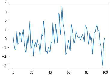
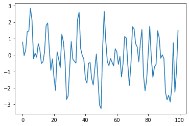
ma_sim = ar_simulater.generate_sample(nsample=100)import matplotlib.pyplot as plt
plt.plot(ma_sim)[<matplotlib.lines.Line2D at 0x2b377d21160>]
Viewing the ACF or PACF
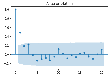
When trying to model ARMA models, we usually use the ACF or PACF. It is worth noting that before this, you will want to have remove trend and seasonality. We will have a full article on ARIMA modeling later on. For MR models, the ACF will help us determine the component, but we also need to confirm the PACF does not drop off as well.
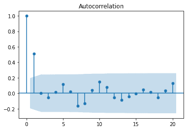
We start with the ACF plot. We see a drastic drop off after the first lag.
from statsmodels.graphics import tsaplots

tsaplots.plot_acf(ma_sim)
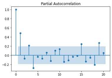
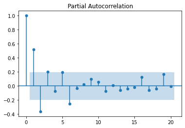
We now look at the PACF plot. We don't see an immediate drop off and later lags seem to be correlated. This is consistent for an MA model.
from statsmodels.graphics import tsaplots

tsaplots.plot_pacf(ma_sim)
Fitting the Model
We can use the built in arima function to model our data. We pass in our data set and the order we want to model.
## Ignore some warnings

import warnings
warnings.filterwarnings('ignore')
from statsmodels.tsa.arima_model import ARMA
mod = ARMA(ma_sim, order=(0, 1))
res = mod.fit()
res.summary()| Dep. Variable: | y | No. Observations: | 100 |
|---|---|---|---|
| Model: | ARMA(0, 1) | Log Likelihood | -142.178 |
| Method: | css-mle | S.D. of innovations | 1.000 |
| Date: | Mon, 09 Aug 2021 | AIC | 290.355 |
| Time: | 07:30:10 | BIC | 298.171 |
| Sample: | 0 | HQIC | 293.518 |
| coef | std err | z | P>|z| | [0.025 | 0.975] | |
|---|---|---|---|---|---|---|
| const | -0.0273 | 0.163 | -0.168 | 0.867 | -0.347 | 0.292 |
| ma.L1.y | 0.6366 | 0.093 | 6.830 | 0.000 | 0.454 | 0.819 |
| Real | Imaginary | Modulus | Frequency | |
|---|---|---|---|---|
| MA.1 | -1.5709 | +0.0000j | 1.5709 | 0.5000 |
We can see the ar1 was modeled at .68 which is very close to the .7 we simulated. Another value to check here is the aic, 147.11, which we would use to confirm the model compared to others.
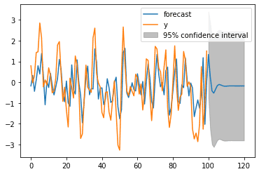
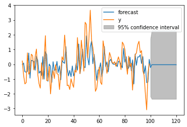
We can now forecast our model using the plot_predict function. Here we predict 20 time values forward and plot the new values.
res.plot_predict(start=0, end = 120)
Modeling an MA(2)
Let's finish with one more example. We will go a bit quick, and use all the steps above.
- Get our data
from statsmodels.tsa.arima_process import ArmaProcess
import numpy as np

ar2 = np.array([1])
ma2 = np.array([1, -.7, .4])

ma2_simulater = ArmaProcess(ar2, ma2)
ma2_sim = ar_simulater.generate_sample(nsample=100)
import matplotlib.pyplot as plt
plt.plot(ma2_sim)[<matplotlib.lines.Line2D at 0x2b38238a5e0>]
- Plot the ACF and PACF
from statsmodels.graphics import tsaplots

tsaplots.plot_acf(ma2_sim)
tsaplots.plot_pacf(ma2_sim)
- Fit and Predict
from statsmodels.tsa.arima_model import ARMA

mod = ARMA(ma2_sim, order=(2, 0))
res = mod.fit()
res.summary()| Dep. Variable: | y | No. Observations: | 100 |
|---|---|---|---|
| Model: | ARMA(2, 0) | Log Likelihood | -147.638 |
| Method: | css-mle | S.D. of innovations | 1.056 |
| Date: | Mon, 09 Aug 2021 | AIC | 303.276 |
| Time: | 07:30:58 | BIC | 313.697 |
| Sample: | 0 | HQIC | 307.494 |
| coef | std err | z | P>|z| | [0.025 | 0.975] | |
|---|---|---|---|---|---|---|
| const | -0.1790 | 0.161 | -1.113 | 0.266 | -0.494 | 0.136 |
| ar.L1.y | 0.7198 | 0.094 | 7.651 | 0.000 | 0.535 | 0.904 |
| ar.L2.y | -0.3770 | 0.093 | -4.033 | 0.000 | -0.560 | -0.194 |
| Real | Imaginary | Modulus | Frequency | |
|---|---|---|---|---|
| AR.1 | 0.9546 | -1.3195j | 1.6286 | -0.1503 |
| AR.2 | 0.9546 | +1.3195j | 1.6286 | 0.1503 |
res.plot_predict(start=0, end = 120)