Boosted Tree Regression in R
06.27.2021
Intro
Boosted Trees are commonly used in regression. They are an ensemble method similar to bagging, however, instead of building mutliple trees in parallel, they build tress sequentially. They used the previous tree to find errors and build a new tree by correcting the previous. In this article, we will learn how to use boosted trees in R.
Data
For this tutorial, we will use the Boston data set which includes
housing data with features of the houses and their prices. We would like
to predict the medv column or the medium value.
library(MASS)
data(Boston)

str(Boston)
## 'data.frame': 506 obs. of 14 variables:
## $ crim : num 0.00632 0.02731 0.02729 0.03237 0.06905 ...
## $ zn : num 18 0 0 0 0 0 12.5 12.5 12.5 12.5 ...
## $ indus : num 2.31 7.07 7.07 2.18 2.18 2.18 7.87 7.87 7.87 7.87 ...
## $ chas : int 0 0 0 0 0 0 0 0 0 0 ...
## $ nox : num 0.538 0.469 0.469 0.458 0.458 0.458 0.524 0.524 0.524 0.524 ...
## $ rm : num 6.58 6.42 7.18 7 7.15 ...
## $ age : num 65.2 78.9 61.1 45.8 54.2 58.7 66.6 96.1 100 85.9 ...
## $ dis : num 4.09 4.97 4.97 6.06 6.06 ...
## $ rad : int 1 2 2 3 3 3 5 5 5 5 ...
## $ tax : num 296 242 242 222 222 222 311 311 311 311 ...
## $ ptratio: num 15.3 17.8 17.8 18.7 18.7 18.7 15.2 15.2 15.2 15.2 ...
## $ black : num 397 397 393 395 397 ...
## $ lstat : num 4.98 9.14 4.03 2.94 5.33 ...
## $ medv : num 24 21.6 34.7 33.4 36.2 28.7 22.9 27.1 16.5 18.9 ...Boosted Tree Regression Model in R
To create a basic Boosted Tree model in R, we can use the gbm function
from the gbm function. We pass the formula of the model medv ~.
which means to model medium value by all other predictors. We also pass
our data Boston.
library(gbm)## Warning: package 'gbm' was built under R version 4.0.5
## Loaded gbm 2.1.8model = gbm(medv ~ ., data = Boston)## Distribution not specified, assuming gaussian ...model## gbm(formula = medv ~ ., data = Boston)
## A gradient boosted model with gaussian loss function.
## 100 iterations were performed.
## There were 13 predictors of which 11 had non-zero influence.Modeling Random Forest in R with Caret
We will now see how to model a ridge regression using the Caret
package. We will use this library as it provides us with many features
for real life modeling. To do this, we use the train method. We pass
the same parameters as above, but in addition we pass the
method = 'rf' model to tell Caret to use a lasso model.
library(caret)## Loading required package: lattice
## Loading required package: ggplot2set.seed(1)
model <- train(
medv ~ .,
data = Boston,
method = 'gbm',
verbose = FALSE
)
model## Stochastic Gradient Boosting
##
## 506 samples
## 13 predictor
##
## No pre-processing
## Resampling: Bootstrapped (25 reps)
## Summary of sample sizes: 506, 506, 506, 506, 506, 506, ...
## Resampling results across tuning parameters:
##
## interaction.depth n.trees RMSE Rsquared MAE
## 1 50 4.299301 0.7856115 2.961434
## 1 100 4.001161 0.8087040 2.720027
## 1 150 3.906931 0.8172835 2.659142
## 2 50 3.919651 0.8170021 2.663399
## 2 100 3.707994 0.8350217 2.513220
## 2 150 3.610815 0.8437581 2.453752
## 3 50 3.773253 0.8298433 2.554777
## 3 100 3.571458 0.8468373 2.419645
## 3 150 3.487586 0.8540058 2.363876
##
## Tuning parameter 'shrinkage' was held constant at a value of 0.1
##
## Tuning parameter 'n.minobsinnode' was held constant at a value of 10
## RMSE was used to select the optimal model using the smallest value.
## The final values used for the model were n.trees = 150, interaction.depth =
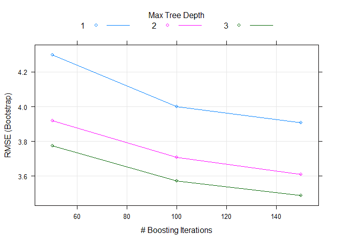
## 3, shrinkage = 0.1 and n.minobsinnode = 10.Here we can see that caret automatically trained over multiple hyper parameters. We can easily plot those to visualize.
plot(model)
Preprocessing with Caret
One feature that we use from Caret is preprocessing. Often in real life
data science we want to run some pre processing before modeling. We will
center and scale our data by passing the following to the train method:
preProcess = c("center", "scale").
set.seed(1)

model2 <- train(
  medv ~ .,
  data = Boston,
  method = 'gbm',
  preProcess = c("center", "scale"),
  verbose = FALSE
)
model2
## Stochastic Gradient Boosting
##
## 506 samples
## 13 predictor
##
## Pre-processing: centered (13), scaled (13)
## Resampling: Bootstrapped (25 reps)
## Summary of sample sizes: 506, 506, 506, 506, 506, 506, ...
## Resampling results across tuning parameters:
##
## interaction.depth n.trees RMSE Rsquared MAE
## 1 50 4.298364 0.7857483 2.960456
## 1 100 4.001210 0.8087314 2.720532
## 1 150 3.907884 0.8171852 2.660320
## 2 50 3.920780 0.8168829 2.663745
## 2 100 3.710591 0.8347560 2.514273
## 2 150 3.613440 0.8434449 2.454870
## 3 50 3.772719 0.8299058 2.555411
## 3 100 3.575442 0.8465749 2.421552
## 3 150 3.493455 0.8536318 2.368105
##
## Tuning parameter 'shrinkage' was held constant at a value of 0.1
##
## Tuning parameter 'n.minobsinnode' was held constant at a value of 10
## RMSE was used to select the optimal model using the smallest value.
## The final values used for the model were n.trees = 150, interaction.depth =
## 3, shrinkage = 0.1 and n.minobsinnode = 10.Splitting the Data Set
Often when we are modeling, we want to split our data into a train and
test set. This way, we can check for overfitting. We can use the
createDataPartition method to do this. In this example, we use the
target medv to split into an 80/20 split, p = .80.
This function will return indexes that contains 80% of the data that we should use for training. We then use the indexes to get our training data from the data set.
set.seed(1)

inTraining <- createDataPartition(Boston$medv, p = .80, list = FALSE)
training <- Boston[inTraining,]
testing  <- Boston[-inTraining,]
We can then fit our model again using only the training data.
set.seed(1)
model3 <- train(
  medv ~ .,
  data = training,
  method = 'gbm',
  preProcess = c("center", "scale"),
  verbose = FALSE
)
model3
## Stochastic Gradient Boosting
##
## 407 samples
## 13 predictor
##
## Pre-processing: centered (13), scaled (13)
## Resampling: Bootstrapped (25 reps)
## Summary of sample sizes: 407, 407, 407, 407, 407, 407, ...
## Resampling results across tuning parameters:
##
## interaction.depth n.trees RMSE Rsquared MAE
## 1 50 4.453135 0.7634033 3.061426
## 1 100 4.194544 0.7858750 2.839732
## 1 150 4.111032 0.7942141 2.768220
## 2 50 4.131221 0.7918313 2.762497
## 2 100 3.940413 0.8103673 2.638015
## 2 150 3.868601 0.8176659 2.604143
## 3 50 4.003287 0.8040027 2.656996
## 3 100 3.831292 0.8203060 2.555678
## 3 150 3.766739 0.8266814 2.518880
##
## Tuning parameter 'shrinkage' was held constant at a value of 0.1
##
## Tuning parameter 'n.minobsinnode' was held constant at a value of 10
## RMSE was used to select the optimal model using the smallest value.
## The final values used for the model were n.trees = 150, interaction.depth =
## 3, shrinkage = 0.1 and n.minobsinnode = 10.Now, we want to check our data on the test set. We can use the subset
method to get the features and test target. We then use the predict
method passing in our model from above and the test features.
Finally, we calculate the RMSE and r2 to compare to the model above.
test.features = subset(testing, select=-c(medv))
test.target = subset(testing, select=medv)[,1]

predictions = predict(model3, newdata = test.features)

# RMSE
sqrt(mean((test.target - predictions)^2))
## [1] 2.323701# R2
cor(test.target, predictions) ^ 2## [1] 0.9386869Cross Validation
In practice, we don’t normal build our data in on training set. It is
common to use a data partitioning strategy like k-fold cross-validation
that resamples and splits our data many times. We then train the model
on these samples and pick the best model. Caret makes this easy with the
trainControl method.
We will use 10-fold cross-validation in this tutorial. To do this we
need to pass three parameters method = "cv", number = 10 (for
10-fold). We store this result in a variable.
set.seed(1)
ctrl <- trainControl(
  method = "cv",
  number = 10
)
Now, we can retrain our model and pass the ctrl response to the
trControl parameter. Notice the our call has added
trControl = set.seed.
# set.seed(1)
model4 <- train(
  medv ~ .,
  data = training,
  method = 'gbm',
  preProcess = c("center", "scale"),
  trControl = ctrl,
  verbose = FALSE
)
model4
## Stochastic Gradient Boosting
##
## 407 samples
## 13 predictor
##
## Pre-processing: centered (13), scaled (13)
## Resampling: Cross-Validated (10 fold)
## Summary of sample sizes: 367, 366, 367, 366, 365, 367, ...
## Resampling results across tuning parameters:
##
## interaction.depth n.trees RMSE Rsquared MAE
## 1 50 4.282246 0.7903540 2.997650
## 1 100 3.949855 0.8146984 2.751481
## 1 150 3.830093 0.8237451 2.677659
## 2 50 3.889972 0.8173126 2.724550
## 2 100 3.640255 0.8382051 2.578475
## 2 150 3.500089 0.8499942 2.483309
## 3 50 3.754281 0.8311812 2.569763
## 3 100 3.509715 0.8506978 2.468093
## 3 150 3.406420 0.8567949 2.419864
##
## Tuning parameter 'shrinkage' was held constant at a value of 0.1
##
## Tuning parameter 'n.minobsinnode' was held constant at a value of 10
## RMSE was used to select the optimal model using the smallest value.
## The final values used for the model were n.trees = 150, interaction.depth =
## 3, shrinkage = 0.1 and n.minobsinnode = 10.plot(model4)
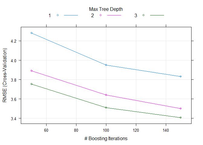
This results seemed to have improved our accuracy for our training data. Let’s check this on the test data to see the results.
test.features = subset(testing, select=-c(medv))
test.target = subset(testing, select=medv)[,1]

predictions = predict(model4, newdata = test.features)

# RMSE
sqrt(mean((test.target - predictions)^2))
## [1] 2.544# R2
cor(test.target, predictions) ^ 2## [1] 0.9264835Tuning Hyper Parameters
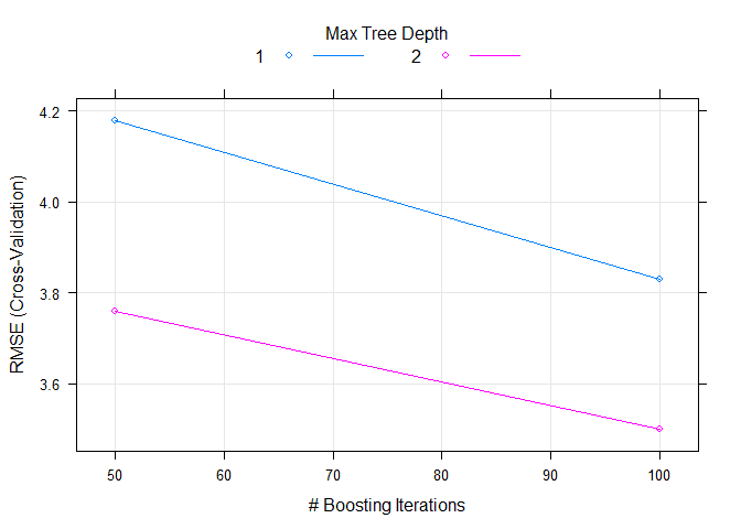
To tune a boosted tree model, we can give the model different values of the tuning parameters. Caret will retrain the model using different tuning params and select the best version.
set.seed(1)

tuneGrid <- expand.grid(
 n.trees = c(50, 100),
 interaction.depth = c(1, 2),
 shrinkage = 0.1,
 n.minobsinnode = 10
)

model5 <- train(
  medv ~ .,
  data = Boston,
  method = 'gbm',
  preProcess = c("center", "scale"),
  trControl = ctrl,
  tuneGrid = tuneGrid,
  verbose = FALSE
)
model5
## Stochastic Gradient Boosting
##
## 506 samples
## 13 predictor
##
## Pre-processing: centered (13), scaled (13)
## Resampling: Cross-Validated (10 fold)
## Summary of sample sizes: 458, 455, 455, 455, 456, 455, ...
## Resampling results across tuning parameters:
##
## interaction.depth n.trees RMSE Rsquared MAE
## 1 50 4.179741 0.7901103 2.899745
## 1 100 3.830113 0.8166134 2.650800
## 2 50 3.758812 0.8272091 2.556187
## 2 100 3.499759 0.8481032 2.391490
##
## Tuning parameter 'shrinkage' was held constant at a value of 0.1
##
## Tuning parameter 'n.minobsinnode' was held constant at a value of 10
## RMSE was used to select the optimal model using the smallest value.
## The final values used for the model were n.trees = 100, interaction.depth =
## 2, shrinkage = 0.1 and n.minobsinnode = 10.Finally, we can again plot the model to see how it performs over different tuning parameters.
plot(model5)