Decision Tree Regression in R

Intro

Decision Trees model regression problems by split data based on different values. This ends by creating a tree structure that you can follow to find the solution. In this article, we will learn how to create Decision Trees in R.

Data

For this tutorial, we will use the Boston data set which includes housing data with features of the houses and their prices. We would like to predict the medv column or the medium value.

library(MASS)
data(Boston)

str(Boston)

## 'data.frame':    506 obs. of  14 variables:
##  $ crim   : num  0.00632 0.02731 0.02729 0.03237 0.06905 ...
##  $ zn     : num  18 0 0 0 0 0 12.5 12.5 12.5 12.5 ...
##  $ indus  : num  2.31 7.07 7.07 2.18 2.18 2.18 7.87 7.87 7.87 7.87 ...
##  $ chas   : int  0 0 0 0 0 0 0 0 0 0 ...
##  $ nox    : num  0.538 0.469 0.469 0.458 0.458 0.458 0.524 0.524 0.524 0.524 ...
##  $ rm     : num  6.58 6.42 7.18 7 7.15 ...
##  $ age    : num  65.2 78.9 61.1 45.8 54.2 58.7 66.6 96.1 100 85.9 ...
##  $ dis    : num  4.09 4.97 4.97 6.06 6.06 ...
##  $ rad    : int  1 2 2 3 3 3 5 5 5 5 ...
##  $ tax    : num  296 242 242 222 222 222 311 311 311 311 ...
##  $ ptratio: num  15.3 17.8 17.8 18.7 18.7 18.7 15.2 15.2 15.2 15.2 ...
##  $ black  : num  397 397 393 395 397 ...
##  $ lstat  : num  4.98 9.14 4.03 2.94 5.33 ...
##  $ medv   : num  24 21.6 34.7 33.4 36.2 28.7 22.9 27.1 16.5 18.9 ...

Basic Decision Tree Regression Model in R

To create a basic Decision Tree regression model in R, we can use the rpart function from the rpart function. We pass the formula of the model medv ~. which means to model medium value by all other predictors. We also pass our data Boston.

library(rpart)
model = rpart(medv ~ ., data = Boston)
model

## n= 506 
## 
## node), split, n, deviance, yval
##       * denotes terminal node
## 
##  1) root 506 42716.3000 22.53281  
##    2) rm< 6.941 430 17317.3200 19.93372  
##      4) lstat>=14.4 175  3373.2510 14.95600  
##        8) crim>=6.99237 74  1085.9050 11.97838 *
##        9) crim< 6.99237 101  1150.5370 17.13762 *
##      5) lstat< 14.4 255  6632.2170 23.34980  
##       10) dis>=1.5511 248  3658.3930 22.93629  
##         20) rm< 6.543 193  1589.8140 21.65648 *
##         21) rm>=6.543 55   643.1691 27.42727 *
##       11) dis< 1.5511 7  1429.0200 38.00000 *
##    3) rm>=6.941 76  6059.4190 37.23816  
##      6) rm< 7.437 46  1899.6120 32.11304  
##       12) lstat>=9.65 7   432.9971 23.05714 *
##       13) lstat< 9.65 39   789.5123 33.73846 *
##      7) rm>=7.437 30  1098.8500 45.09667 *

Modeling Decision Regression in R with Caret

We will now see how to model a ridge regression using the Caret package. We will use this library as it provides us with many features for real life modeling. To do this, we use the train method. We pass the same parameters as above, but in addition we pass the method = 'rpart2' model to tell Caret to use a lasso model.

library(caret)

## Loading required package: lattice

## Loading required package: ggplot2

set.seed(1)

model <- train(
  medv ~ .,
  data = Boston,
  method = 'rpart2'
)
model

## CART 
## 
## 506 samples
##  13 predictor
## 
## No pre-processing
## Resampling: Bootstrapped (25 reps) 
## Summary of sample sizes: 506, 506, 506, 506, 506, 506, ... 
## Resampling results across tuning parameters:
## 
##   maxdepth  RMSE      Rsquared   MAE     
##   1         7.205170  0.3878083  5.350946
##   2         6.093925  0.5626475  4.384026
##   3         5.041290  0.6997700  3.491774
## 
## RMSE was used to select the optimal model using the smallest value.
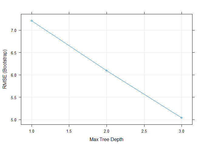
## The final value used for the model was maxdepth = 3.

Here we can see that caret automatically trained over multiple hyper parameters. We can easily plot those to visualize.

plot(model)

Preprocessing with Caret

One feature that we use from Caret is preprocessing. Often in real life data science we want to run some pre processing before modeling. We will center and scale our data by passing the following to the train method: preProcess = c("center", "scale").

set.seed(1)

model2 <- train(
  medv ~ .,
  data = Boston,
  method = 'rpart2',
  preProcess = c("center", "scale")
)
model2

## CART 
## 
## 506 samples
##  13 predictor
## 
## Pre-processing: centered (13), scaled (13) 
## Resampling: Bootstrapped (25 reps) 
## Summary of sample sizes: 506, 506, 506, 506, 506, 506, ... 
## Resampling results across tuning parameters:
## 
##   maxdepth  RMSE      Rsquared   MAE     
##   1         7.204223  0.3880450  5.349965
##   2         6.091834  0.5629676  4.381820
##   3         5.040201  0.6999240  3.490292
## 
## RMSE was used to select the optimal model using the smallest value.
## The final value used for the model was maxdepth = 3.

Splitting the Data Set

Often when we are modeling, we want to split our data into a train and test set. This way, we can check for overfitting. We can use the createDataPartition method to do this. In this example, we use the target medv to split into an 80/20 split, p = .80.

This function will return indexes that contains 80% of the data that we should use for training. We then use the indexes to get our training data from the data set.

set.seed(1)

inTraining <- createDataPartition(Boston$medv, p = .80, list = FALSE)
training <- Boston[inTraining,]
testing  <- Boston[-inTraining,]

We can then fit our model again using only the training data.

set.seed(1)
model3 <- train(
  medv ~ .,
  data = training,
  method = 'rpart2',
  preProcess = c("center", "scale")
)
model3

## CART 
## 
## 407 samples
##  13 predictor
## 
## Pre-processing: centered (13), scaled (13) 
## Resampling: Bootstrapped (25 reps) 
## Summary of sample sizes: 407, 407, 407, 407, 407, 407, ... 
## Resampling results across tuning parameters:
## 
##   maxdepth  RMSE      Rsquared   MAE     
##   1         7.113422  0.4023752  5.324373
##   2         6.022926  0.5704029  4.348765
##   3         5.176067  0.6821559  3.579060
## 
## RMSE was used to select the optimal model using the smallest value.
## The final value used for the model was maxdepth = 3.

Now, we want to check our data on the test set. We can use the subset method to get the features and test target. We then use the predict method passing in our model from above and the test features.

Finally, we calculate the RMSE and r2 to compare to the model above.

test.features = subset(testing, select=-c(medv))
test.target = subset(testing, select=medv)[,1]

predictions = predict(model3, newdata = test.features)

# RMSE
sqrt(mean((test.target - predictions)^2))

## [1] 4.295796

# R2
cor(test.target, predictions) ^ 2

## [1] 0.792355

Cross Validation

In practice, we don’t normal build our data in on training set. It is common to use a data partitioning strategy like k-fold cross-validation that resamples and splits our data many times. We then train the model on these samples and pick the best model. Caret makes this easy with the trainControl method.

We will use 10-fold cross-validation in this tutorial. To do this we need to pass three parameters method = "cv", number = 10 (for 10-fold). We store this result in a variable.

set.seed(1)
ctrl <- trainControl(
  method = "cv",
  number = 10,
)

Now, we can retrain our model and pass the ctrl response to the trControl parameter. Notice the our call has added trControl = set.seed.

# set.seed(1)
model4 <- train(
  medv ~ .,
  data = training,
  method = 'rpart2',
  preProcess = c("center", "scale"),
  trControl = ctrl
)
model4

## CART 
## 
## 407 samples
##  13 predictor
## 
## Pre-processing: centered (13), scaled (13) 
## Resampling: Cross-Validated (10 fold) 
## Summary of sample sizes: 367, 366, 367, 366, 365, 367, ... 
## Resampling results across tuning parameters:
## 
##   maxdepth  RMSE      Rsquared   MAE     
##   1         7.019771  0.4286280  5.201582
##   2         5.940912  0.5940990  4.262869
##   3         4.825295  0.7249753  3.364939
## 
## RMSE was used to select the optimal model using the smallest value.
## The final value used for the model was maxdepth = 3.

plot(model4)

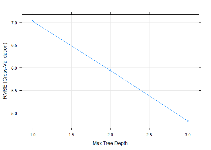
This results seemed to have improved our accuracy for our training data. Let’s check this on the test data to see the results.

test.features = subset(testing, select=-c(medv))
test.target = subset(testing, select=medv)[,1]

predictions = predict(model4, newdata = test.features)

# RMSE
sqrt(mean((test.target - predictions)^2))

## [1] 4.295796

# R2
cor(test.target, predictions) ^ 2

## [1] 0.792355

Tuning Hyper Parameters

To tune a ridge model, we can give the model different values of lambda. Caret will retrain the model using different lambdas and select the best version.

set.seed(1)

tuneGrid <- expand.grid(
  degree = 1, 
  nprune = c(2, 11, 10)
)

model5 <- train(
  medv ~ .,
  data = training,
  method = 'earth',
  preProcess = c("center", "scale"),
  trControl = ctrl,
  tuneGrid = tuneGrid
)

## Loading required package: earth

## Warning: package 'earth' was built under R version 4.0.5

## Loading required package: Formula

## Loading required package: plotmo

## Warning: package 'plotmo' was built under R version 4.0.5

## Loading required package: plotrix

## Loading required package: TeachingDemos

## Warning: package 'TeachingDemos' was built under R version 4.0.5

model5

## Multivariate Adaptive Regression Spline 
## 
## 407 samples
##  13 predictor
## 
## Pre-processing: centered (13), scaled (13) 
## Resampling: Cross-Validated (10 fold) 
## Summary of sample sizes: 367, 366, 367, 366, 365, 367, ... 
## Resampling results across tuning parameters:
## 
##   nprune  RMSE      Rsquared   MAE     
##    2      6.172609  0.5477370  4.504196
##   10      4.014690  0.8120098  2.837775
##   11      3.933227  0.8191702  2.794837
## 
## Tuning parameter 'degree' was held constant at a value of 1
## RMSE was used to select the optimal model using the smallest value.
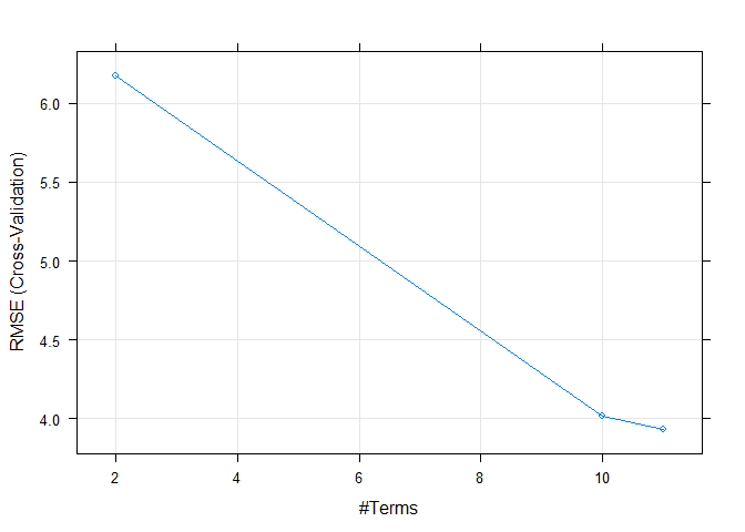
## The final values used for the model were nprune = 11 and degree = 1.

Finally, we can again plot the model to see how it performs over different tuning parameters.

plot(model5)