How to Create a ggplot2 Dot Plot in R

Intro

A dot plot is similar to a histogram except each plot represents a single observation. This kind of plot allows you to see individual observations and their relationships while see the summary statistic as well. In this article, we will learn how to create dot plots with ggplot2.

For those with little time

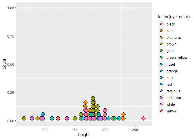
For those who are in a hurry, here is a common example with separation by factors.

library(tidyverse)

## -- Attaching packages --------------------------------------- tidyverse 1.3.1 --

## v ggplot2 3.3.3     v purrr   0.3.4
## v tibble  3.1.0     v dplyr   1.0.5
## v tidyr   1.1.3     v stringr 1.4.0
## v readr   1.4.0     v forcats 0.5.1

## -- Conflicts ------------------------------------------ tidyverse_conflicts() --
## x dplyr::filter() masks stats::filter()
## x dplyr::lag()    masks stats::lag()

data(starwars, package = 'dplyr')

ggplot(starwars, aes(x = height, fill = factor(eye_color))) + geom_dotplot()

## `stat_bindot()` using `bins = 30`. Pick better value with `binwidth`.

Loading the data

We begin by loading our data set. I like to use the starwars data set that is released in the dyplr, because it is fun :D.

data(starwars, package = 'dplyr')

print(starwars)

## # A tibble: 87 x 14
##    name    height  mass hair_color  skin_color eye_color birth_year sex   gender
##    <chr>    <int> <dbl> <chr>       <chr>      <chr>          <dbl> <chr> <chr> 
##  1 Luke S~    172    77 blond       fair       blue            19   male  mascu~
##  2 C-3PO      167    75 <NA>        gold       yellow         112   none  mascu~
##  3 R2-D2       96    32 <NA>        white, bl~ red             33   none  mascu~
##  4 Darth ~    202   136 none        white      yellow          41.9 male  mascu~
##  5 Leia O~    150    49 brown       light      brown           19   fema~ femin~
##  6 Owen L~    178   120 brown, grey light      blue            52   male  mascu~
##  7 Beru W~    165    75 brown       light      blue            47   fema~ femin~
##  8 R5-D4       97    32 <NA>        white, red red             NA   none  mascu~
##  9 Biggs ~    183    84 black       light      brown           24   male  mascu~
## 10 Obi-Wa~    182    77 auburn, wh~ fair       blue-gray       57   male  mascu~
## # ... with 77 more rows, and 5 more variables: homeworld <chr>, species <chr>,
## #   films <list>, vehicles <list>, starships <list>

Creating the Basic Dot Plot

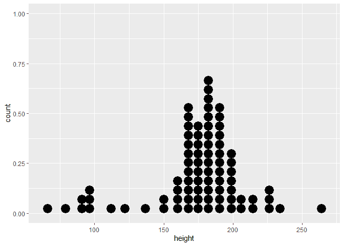
To create a basic dot plot with ggplot2, we can use the geom_dotplot geometry function.

library(tidyverse)
ggplot(starwars, aes(x = height)) + geom_dotplot()

## `stat_bindot()` using `bins = 30`. Pick better value with `binwidth`.

## Warning: Removed 6 rows containing non-finite values (stat_bindot).

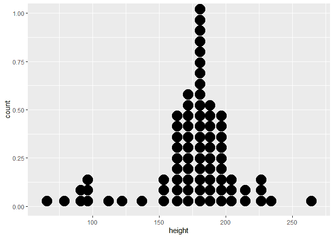
Selecting the Bin Width

The binwidth is determined by default using a density selecting algorithm. We can set a max width by using the binwidth option.

ggplot(starwars, aes(x = height)) + geom_dotplot(binwidth = 8)

## Warning: Removed 6 rows containing non-finite values (stat_bindot).

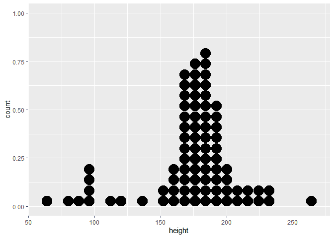
We can also use the method="histodot" to fix the width of the bins.

ggplot(starwars, aes(x = height)) + geom_dotplot(method="histodot", binwidth = 8)

## Warning: Removed 6 rows containing non-finite values (stat_bindot).

Changing the Stacking

We can also use the stackdir to alter how the data is stacked. Here is an example of center stacking.

ggplot(starwars, aes(x = height)) + geom_dotplot(stackdir = "center")

## `stat_bindot()` using `bins = 30`. Pick better value with `binwidth`.

## Warning: Removed 6 rows containing non-finite values (stat_bindot).

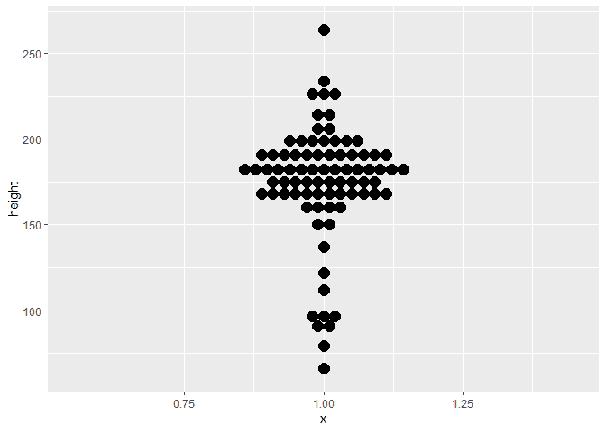
We can also change the direction of the stacking to the y-axis with the binaxis option. We also need to set the x = 1 and the y = to our height.

ggplot(starwars, aes(x = 1, y = height)) + geom_dotplot(binaxis = "y", stackdir = "center")

## `stat_bindot()` using `bins = 30`. Pick better value with `binwidth`.

## Warning: Removed 6 rows containing non-finite values (stat_bindot).

Altering the Dot Styles

If we would like to alter the styles of the dots, we have a few options. First, we can change the size.

ggplot(starwars, aes(x = height)) + geom_dotplot(dotsize = 1.5)

## `stat_bindot()` using `bins = 30`. Pick better value with `binwidth`.

## Warning: Removed 6 rows containing non-finite values (stat_bindot).

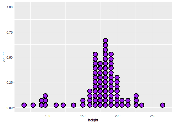
We can also change the fill and stroke.

ggplot(starwars, aes(x = height)) + geom_dotplot(fill = "purple", stroke = 3)

## `stat_bindot()` using `bins = 30`. Pick better value with `binwidth`.

## Warning: Removed 6 rows containing non-finite values (stat_bindot).

Separating by Factor

We can also color or separate the data by factor. Let’s check the different heights by eye color to see if their may be any relation. We can use the fill property in the aes to accomplish this.

ggplot(starwars, aes(x = height, fill = factor(eye_color))) + geom_dotplot()

## `stat_bindot()` using `bins = 30`. Pick better value with `binwidth`.

## Warning: Removed 6 rows containing non-finite values (stat_bindot).