How to Create a ggplot Histogram Plot in R

Intro

Histogram plots allow you to view distributions of continuous variables. The plot will bin a continuous variable into groups and count the number of observations in each group. This helps you few the distribution and see if it fits a common probability distribution. In this article, we will learn how to create ggplot Histograms in R.

If you are in a rush

For those with little time, here is a quick snippet of box plots. Read on for more details.

library(ggplot2)
data(starwars, package = 'dplyr')

ggplot(starwars, aes(x = height, colour = sex, fill = sex)) +
  geom_histogram()

## `stat_bin()` using `bins = 30`. Pick better value with `binwidth`.

Loading the data

For our tutorial, we will use the starwars data set from the dplyr package.

library(tidyverse)

data(starwars, package = 'dplyr')

glimpse(starwars)

## Rows: 87
## Columns: 14
## $ name       <chr> "Luke Skywalker", "C-3PO", "R2-D2", "Darth Vader", "Leia Or~
## $ height     <int> 172, 167, 96, 202, 150, 178, 165, 97, 183, 182, 188, 180, 2~
## $ mass       <dbl> 77.0, 75.0, 32.0, 136.0, 49.0, 120.0, 75.0, 32.0, 84.0, 77.~
## $ hair_color <chr> "blond", NA, NA, "none", "brown", "brown, grey", "brown", N~
## $ skin_color <chr> "fair", "gold", "white, blue", "white", "light", "light", "~
## $ eye_color  <chr> "blue", "yellow", "red", "yellow", "brown", "blue", "blue",~
## $ birth_year <dbl> 19.0, 112.0, 33.0, 41.9, 19.0, 52.0, 47.0, NA, 24.0, 57.0, ~
## $ sex        <chr> "male", "none", "none", "male", "female", "male", "female",~
## $ gender     <chr> "masculine", "masculine", "masculine", "masculine", "femini~
## $ homeworld  <chr> "Tatooine", "Tatooine", "Naboo", "Tatooine", "Alderaan", "T~
## $ species    <chr> "Human", "Droid", "Droid", "Human", "Human", "Human", "Huma~
## $ films      <list> <"The Empire Strikes Back", "Revenge of the Sith", "Return~
## $ vehicles   <list> <"Snowspeeder", "Imperial Speeder Bike">, <>, <>, <>, "Imp~
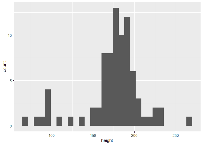
## $ starships  <list> <"X-wing", "Imperial shuttle">, <>, <>, "TIE Advanced x1",~

Building the Basic ggplot Histogram

ggplot(starwars, aes(x = height)) +
  geom_histogram()

## `stat_bin()` using `bins = 30`. Pick better value with `binwidth`.

## Warning: Removed 6 rows containing non-finite values (stat_bin).

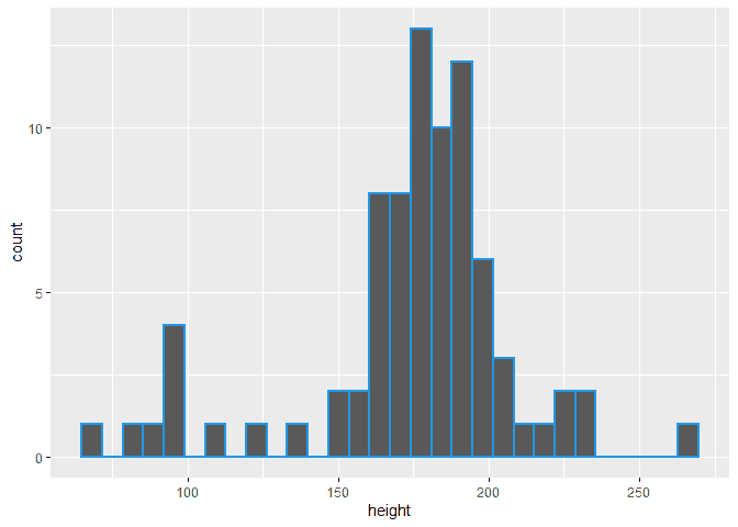
Customizing the ggplot Histogram

ggplot(starwars, aes(x = height)) +
  geom_histogram(color = 4,
               lwd = 1,
               linetype = 1)

## `stat_bin()` using `bins = 30`. Pick better value with `binwidth`.

## Warning: Removed 6 rows containing non-finite values (stat_bin).

ggplot(starwars, aes(x = height)) +
  geom_histogram(color = 4,
               fill = 4,
               alpha = 0.25)

## `stat_bin()` using `bins = 30`. Pick better value with `binwidth`.

## Warning: Removed 6 rows containing non-finite values (stat_bin).

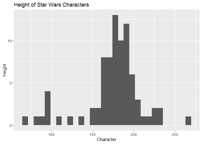
Label

ggplot(starwars, aes(x = height)) +
  geom_histogram() +
  labs(
    title = "Height of Star Wars Characters",
    x = "Character",
    y = "Height"
  )

## `stat_bin()` using `bins = 30`. Pick better value with `binwidth`.

## Warning: Removed 6 rows containing non-finite values (stat_bin).

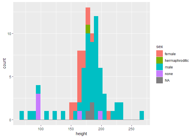
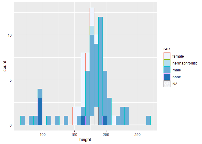
Grouping by Color

library(ggplot2)

ggplot(starwars, aes(x = height, colour = sex, fill = sex)) +
  geom_histogram()

## `stat_bin()` using `bins = 30`. Pick better value with `binwidth`.

## Warning: Removed 6 rows containing non-finite values (stat_bin).

Facets and Creating Separate Plots

library(ggplot2)


ggplot(starwars, aes(x = height, colour = sex, fill = sex)) +
  geom_histogram() +
  facet_grid(~sex)

## `stat_bin()` using `bins = 30`. Pick better value with `binwidth`.

## Warning: Removed 6 rows containing non-finite values (stat_bin).

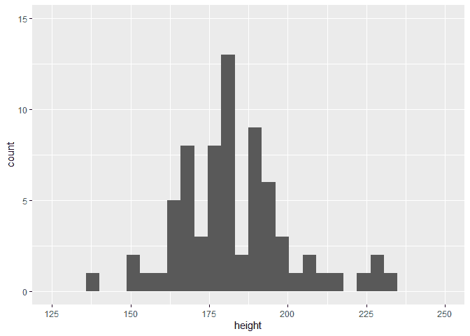
Limiting X and Y

ggplot(starwars, aes(x = height)) +
  geom_histogram() +
  xlim(125, 250) +
  ylim(0, 15)

## `stat_bin()` using `bins = 30`. Pick better value with `binwidth`.

## Warning: Removed 16 rows containing non-finite values (stat_bin).

## Warning: Removed 2 rows containing missing values (geom_bar).

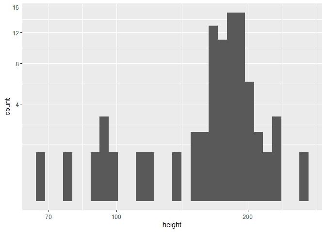
Scaling X and Y

ggplot(starwars, aes(x = height)) +
  geom_histogram() +
  scale_x_log10() +
  scale_y_sqrt()

## `stat_bin()` using `bins = 30`. Pick better value with `binwidth`.

## Warning: Removed 6 rows containing non-finite values (stat_bin).

Color and Fill Scales

library(ggplot2)


ggplot(starwars, aes(x = height, colour = sex, fill = sex)) +
  geom_histogram() +
  scale_fill_brewer()

## `stat_bin()` using `bins = 30`. Pick better value with `binwidth`.

## Warning: Removed 6 rows containing non-finite values (stat_bin).

Customizing the Legend

ggplot(starwars, aes(x = height, colour = sex, fill = sex)) +
  geom_histogram() +
  theme(legend.position="top")

## `stat_bin()` using `bins = 30`. Pick better value with `binwidth`.

## Warning: Removed 6 rows containing non-finite values (stat_bin).

ggplot(starwars, aes(x = height, colour = sex, fill = sex)) +
  geom_histogram() +
  theme(legend.position="bottom")

## `stat_bin()` using `bins = 30`. Pick better value with `binwidth`.

## Warning: Removed 6 rows containing non-finite values (stat_bin).

ggplot(starwars, aes(x = height, colour = sex, fill = sex)) +
  geom_histogram() +
  theme(legend.position="none")

## `stat_bin()` using `bins = 30`. Pick better value with `binwidth`.

## Warning: Removed 6 rows containing non-finite values (stat_bin).

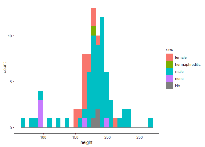
Using Themes

ggplot(starwars, aes(x = height, colour = sex, fill = sex)) +
  geom_histogram() +
  theme_classic()

## `stat_bin()` using `bins = 30`. Pick better value with `binwidth`.

## Warning: Removed 6 rows containing non-finite values (stat_bin).