Time Series Decomposition in R

Intro

When working with time series data, we often want to decompose a time series into several components. We usually want to break out the trend, seasonality, and noise. In this article, we will learn how to decompose a time series in R.

Data

Let’s load a data set of monthly milk production. We will load it from the url below. The data consists of monthly intervals and kilograms of milk produced.

df <- read.csv('https://raw.githubusercontent.com/ourcodingclub/CC-time-series/master/monthly_milk.csv')
df$month = as.Date(df$month)
head(df)

##        month milk_prod_per_cow_kg
## 1 1962-01-01               265.05
## 2 1962-02-01               252.45
## 3 1962-03-01               288.00
## 4 1962-04-01               295.20
## 5 1962-05-01               327.15
## 6 1962-06-01               313.65

Now, we convert our data to a time series object using the R ts method.

df.ts = ts(df[, -1], frequency = 12, start=c(1962, 1, 1))
head(df.ts)

## [1] 265.05 252.45 288.00 295.20 327.15 313.65

Decomposing the Time Series

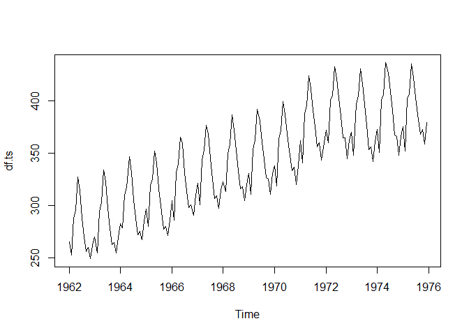
Let’s first plot our time series to see the trend.

plot(df.ts)

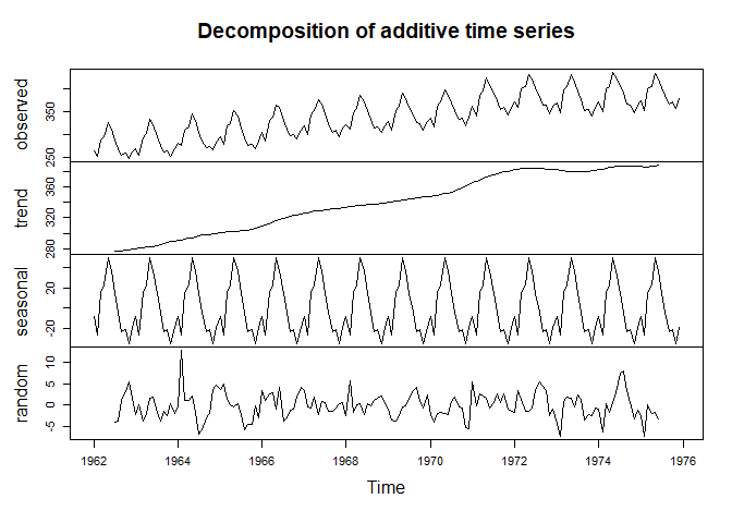
To decompose a time series, we can use the built in decompose function.

dec <- decompose(df.ts)

Now that we have a decomposed object, we can plot to see the separation of seasonal, trend, and residuals.

plot(dec)

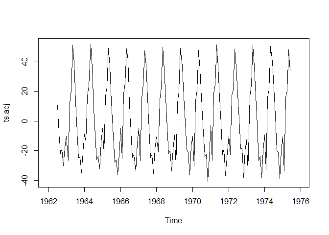
Adjusting the Time Series

Now that we have decomposed the model, let’s say we would like to remove details from our time series. For example, we can subtract the seasonaility as follows.

ts.adj <- df.ts - dec$seasonal
plot(ts.adj)

Similarly with the trend.

ts.adj <- df.ts - dec$trend
plot(ts.adj)