
Simple Exponential Smoothing in Python
07.27.2021
Intro
Simple Exponential Smoothing is a forecasting model that extends the basic moving average by adding weights to previous lags. As the lags grow, the weight, alpha, is decreased which leads to closer lags having more predictive power than farther lags. In this article, we will learn how to create a Simple Exponential Smoothing model in Python.
Data
Let's load a data set of monthly milk production. We will load it from the url below. The data consists of monthly intervals and kilograms of milk produced.
import pandas as pd

df = pd.read_csv('https://raw.githubusercontent.com/ourcodingclub/CC-time-series/master/monthly_milk.csv')

df.month = pd.to_datetime(df.month)
df = df.set_index('month')
df.head()| milk_prod_per_cow_kg | |
|---|---|
| month | |
| 1962-01-01 | 265.05 |
| 1962-02-01 | 252.45 |
| 1962-03-01 | 288.00 |
| 1962-04-01 | 295.20 |
| 1962-05-01 | 327.15 |
Simple Exponential Smoothing in Python
Let's start by plotting our time series.
df.plot()<AxesSubplot:xlabel='month'>
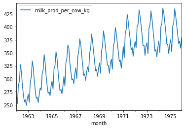
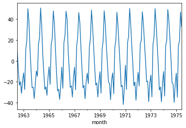
SES assumes that the data has be detrended and seasonaility has been removed, so we will use the seasonal_decompose to remove these from our data. From the graph below, we did an okay job, although we will need to do more processing and testing to be sure. For our purposes, we will use this.
from statsmodels.tsa.seasonal import seasonal_decompose


result = seasonal_decompose(df.milk_prod_per_cow_kg,  model = 'multiplicable')

data = df.milk_prod_per_cow_kg - result.seasonal - result.trend

## Drop the removed
data = data.dropna()

data.plot()
<AxesSubplot:xlabel='month'>
To create a simple exponential smoothing model, we can use the SimpleExpSmoothing from the statsmodels package. We first create an instance of the class with our data, then call the fit method with the value of alpha we want to use.
from statsmodels.tsa.api import SimpleExpSmoothing

ses = SimpleExpSmoothing(data)

alpha = 0.2
model = ses.fit(smoothing_level = alpha, optimized = False)
c:\users\krh12\appdata\local\programs\python\python39\lib\site-packages\statsmodels\tsa\base\tsa_model.py:524: ValueWarning: No frequency information was provided, so inferred frequency MS will be used.
warnings.warn('No frequency information was'
c:\users\krh12\appdata\local\programs\python\python39\lib\site-packages\statsmodels\tsa\holtwinters\model.py:427: FutureWarning: After 0.13 initialization must be handled at model creation
warnings.warn(Now that we have the model, we can forecast using the forcast method. We will predict the next 3 months.
forcast = model.forecast(3)
forcast
c:\users\krh12\appdata\local\programs\python\python39\lib\site-packages\statsmodels\tsa\base\tsa_model.py:132: FutureWarning: The 'freq' argument in Timestamp is deprecated and will be removed in a future version.
date_key = Timestamp(key, freq=base_index.freq)
1975-07-01 11.674527
1975-08-01 11.674527
1975-09-01 11.674527
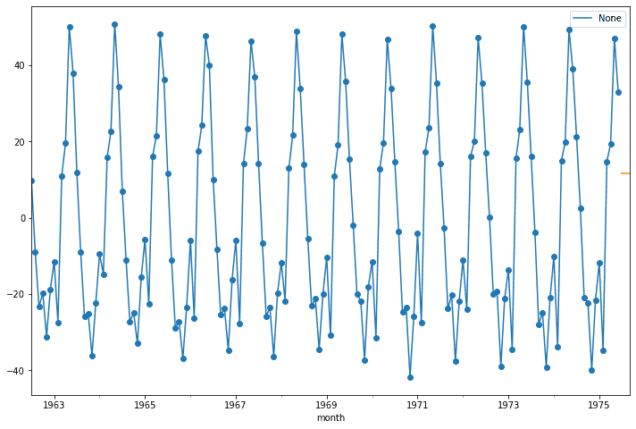
Freq: MS, dtype: float64We can then plot the forcasted with our original data. Unfortunately, the model just predicts three of the same values :P.
ax = data.plot(marker = 'o', figsize = (12,8), legend = True)

forcast.plot(ax = ax)
<AxesSubplot:xlabel='month'>
Simple Exponential Smothing By Hand
SES is a very simple model and helps with understanding future models. With this in mind, I think it is good to try and build these models by hand to help learn the intricate details of models. Learning these simple models will help with the more complex.
The equation for SES is the following:
You can read this equation by saying, the next value of our time series is the previous value plus alpha (our learning rate) times the error of the previous value.
One this to note is we assume the following:
That is, the first predicted value is just the first value in our time series.
We can use a bit of algebra to change the equation above to help with iterative calculations. Let's s.tart with an example of predicting y_3
This gives us a nice form to iterate through an predict data. Let's see why by doing an example. Let's say we have the following data.
| t | y |
|---|---|
| 1 | 3 |
| 2 | 5 |
| 3 | 9 |
| 4 | 20 |
We can apply our model as follows. We will use an alpha of .4.
For t = 1.
Now for t = 2.
For t = 3
For t = 4
Let's finish by writing some simple code to replicate this.
y = [3, 5, 9, 20]

## Start with the first point
forcast = [y[0]]
alpha = .4

for i in range(1, len(y)):
    predict = alpha * y[i - 1] + (1 - alpha) * forcast[i - 1]
    forcast.append(predict)

forcast
3
5
9
[3, 3.0, 3.8, 5.88]