Lasso Regression in R

Intro

Lasso regression is a model that builds on linear regression to solve for issues of multicolinearity. The optimization functin in lasso adds a shrinkage parameter which allows for remove features from the final model. We will look at the math for this model in another article. In this article, we will learn how to perform lasso regression in R.

Data

For this tutorial, we will use the Boston data set which includes housing data with features of the houses and their prices. We would like to predict the medv column or the medium value.

library(MASS)
data(Boston)
str(Boston)

## 'data.frame':    506 obs. of  14 variables:
##  $ crim   : num  0.00632 0.02731 0.02729 0.03237 0.06905 ...
##  $ zn     : num  18 0 0 0 0 0 12.5 12.5 12.5 12.5 ...
##  $ indus  : num  2.31 7.07 7.07 2.18 2.18 2.18 7.87 7.87 7.87 7.87 ...
##  $ chas   : int  0 0 0 0 0 0 0 0 0 0 ...
##  $ nox    : num  0.538 0.469 0.469 0.458 0.458 0.458 0.524 0.524 0.524 0.524 ...
##  $ rm     : num  6.58 6.42 7.18 7 7.15 ...
##  $ age    : num  65.2 78.9 61.1 45.8 54.2 58.7 66.6 96.1 100 85.9 ...
##  $ dis    : num  4.09 4.97 4.97 6.06 6.06 ...
##  $ rad    : int  1 2 2 3 3 3 5 5 5 5 ...
##  $ tax    : num  296 242 242 222 222 222 311 311 311 311 ...
##  $ ptratio: num  15.3 17.8 17.8 18.7 18.7 18.7 15.2 15.2 15.2 15.2 ...
##  $ black  : num  397 397 393 395 397 ...
##  $ lstat  : num  4.98 9.14 4.03 2.94 5.33 ...
##  $ medv   : num  24 21.6 34.7 33.4 36.2 28.7 22.9 27.1 16.5 18.9 ...

Basic Lasso Regression in R

To create a basic lasso regressio model in R, we can use the `enet method from the elasticnet library. We need to supply a fixed lambda parameter as that will be used for ridge regression.

library(elasticnet)

## Loading required package: lars

## Loaded lars 1.2

predictors = subset(Boston, select = -c(medv))
target = subset(Boston, select = medv)[,1]

model = enet(
  x = as.matrix(predictors),
  y = target,
  lambda = 0.001
)
summary(model)

##           Length Class  Mode     
## call        4    -none- call     
## actions    16    -none- list     
## allset     13    -none- numeric  
## beta.pure 208    -none- numeric  
## vn         13    -none- character
## mu          1    -none- numeric  
## normx      13    -none- numeric  
## meanx      13    -none- numeric  
## lambda      1    -none- numeric  
## L1norm     16    -none- numeric  
## penalty    16    -none- numeric  
## df         16    -none- numeric  
## Cp         16    -none- numeric  
## sigma2      1    -none- numeric

Modeling Lasso Regression in R with Caret

We will now see how to model a lasso regression using the Caret package. We will use this library as it provides us with many features for real life modeling.

To do this, we use the train method. We pass the same parameters as above, but in addition we pass the method = 'lasso' model to tell Caret to use a lasso model.

set.seed(1)

library(caret)

## Loading required package: lattice

## Loading required package: ggplot2

model <- train(
  medv ~ .,
  data = Boston,
  method = 'lasso'
)
model

## The lasso 
## 
## 506 samples
##  13 predictor
## 
## No pre-processing
## Resampling: Bootstrapped (25 reps) 
## Summary of sample sizes: 506, 506, 506, 506, 506, 506, ... 
## Resampling results across tuning parameters:
## 
##   fraction  RMSE      Rsquared   MAE     
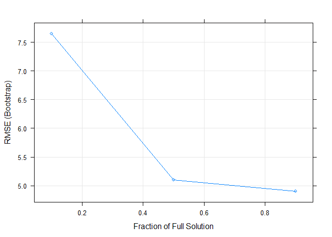
##   0.1       7.644625  0.5958350  5.409666
##   0.5       5.102968  0.6927114  3.507566
##   0.9       4.906142  0.7154243  3.443382
## 
## RMSE was used to select the optimal model using the smallest value.
## The final value used for the model was fraction = 0.9.

Here we can see that caret automatically trained over multiple hyper parameters. We can easily plot those to visualize.

plot(model)

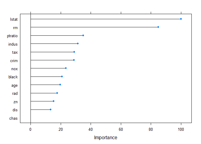
We can also see a graph of the importance plot which will show if the lasso model removed any parameters.

plot(varImp(model))

Preprocessing with Caret

One feature that we use from Caret is preprocessing. Often in real life data science we want to run some pre processing before modeling. We will center and scale our data by passing the following to the train method: preProcess = c("center", "scale").

set.seed(1)

model2 <- train(
  medv ~ .,
  data = Boston,
  method = 'lasso',
  preProcess = c("center", "scale")
)
model2

## The lasso 
## 
## 506 samples
##  13 predictor
## 
## Pre-processing: centered (13), scaled (13) 
## Resampling: Bootstrapped (25 reps) 
## Summary of sample sizes: 506, 506, 506, 506, 506, 506, ... 
## Resampling results across tuning parameters:
## 
##   fraction  RMSE      Rsquared   MAE     
##   0.1       7.644625  0.5958350  5.409666
##   0.5       5.102968  0.6927114  3.507566
##   0.9       4.906142  0.7154243  3.443382
## 
## RMSE was used to select the optimal model using the smallest value.
## The final value used for the model was fraction = 0.9.

Splitting the Data Set

Often when we are modeling, we want to split our data into a train and test set. This way, we can check for overfitting. We can use the createDataPartition method to do this. In this example, we use the target medv to split into an 80/20 split, p = .80.

This function will return indexes that contains 80% of the data that we should use for training. We then use the indexes to get our training data from the data set.

set.seed(1)

inTraining <- createDataPartition(Boston$medv, p = .80, list = FALSE)
training <- Boston[inTraining,]
testing  <- Boston[-inTraining,]

We can then fit our model again using only the training data.

set.seed(1)
model3 <- train(
  medv ~ .,
  data = training,
  method = 'lasso',
  preProcess = c("center", "scale")
)
model3

## The lasso 
## 
## 407 samples
##  13 predictor
## 
## Pre-processing: centered (13), scaled (13) 
## Resampling: Bootstrapped (25 reps) 
## Summary of sample sizes: 407, 407, 407, 407, 407, 407, ... 
## Resampling results across tuning parameters:
## 
##   fraction  RMSE      Rsquared   MAE     
##   0.1       7.589522  0.6175869  5.406797
##   0.5       5.138219  0.6868388  3.534709
##   0.9       4.900645  0.7151607  3.428199
## 
## RMSE was used to select the optimal model using the smallest value.
## The final value used for the model was fraction = 0.9.

Now, we want to check our data on the test set. We can use the subset method to get the features and test target. We then use the predict method passing in our model from above and the test features.

Finally, we calculate the RMSE and r2 to compare to the model above.

test.features = subset(testing, select=-c(medv))
test.target = subset(testing, select=medv)[,1]

predictions = predict(model3, newdata = test.features)

# RMSE
sqrt(mean((test.target - predictions)^2))

## [1] 5.092187

# R2
cor(test.target, predictions) ^ 2

## [1] 0.7133683

Cross Validation

In practice, we don’t normal build our data in on training set. It is common to use a data partitioning strategy like k-fold cross-validation that resamples and splits our data many times. We then train the model on these samples and pick the best model. Caret makes this easy with the trainControl method.

We will use 10-fold cross-validation in this tutorial. To do this we need to pass three parameters method = "repeatedcv", number = 10 (for 10-fold). We store this result in a variable.

set.seed(1)
ctrl <- trainControl(
  method = "cv",
  number = 10,
)

Now, we can retrain our model and pass the trainControl response to the trControl parameter. Notice the our call has added trControl = set.seed.

set.seed(1)

model4 <- train(
  medv ~ .,
  data = training,
  method = 'lasso',
  preProcess = c("center", "scale"),
  trControl = ctrl
)
model4

## The lasso 
## 
## 407 samples
##  13 predictor
## 
## Pre-processing: centered (13), scaled (13) 
## Resampling: Cross-Validated (10 fold) 
## Summary of sample sizes: 367, 366, 367, 366, 365, 367, ... 
## Resampling results across tuning parameters:
## 
##   fraction  RMSE      Rsquared   MAE     
##   0.1       7.611127  0.6223092  5.476068
##   0.5       5.022313  0.7111354  3.578952
##   0.9       4.744846  0.7391371  3.408950
## 
## RMSE was used to select the optimal model using the smallest value.
## The final value used for the model was fraction = 0.9.

This results seemed to have improved our accuracy for our training data. Let’s check this on the test data to see the results.

test.features = subset(testing, select=-c(medv))
test.target = subset(testing, select=medv)[,1]

predictions = predict(model4, newdata = test.features)

# RMSE
sqrt(mean((test.target - predictions)^2))

## [1] 5.092187

# R2
cor(test.target, predictions) ^ 2

## [1] 0.7133683

Tuning Hyper Parameters

With a lasso regression, we can tune the fraction parameter which will control how strong the shrinkage works in the optimization model. To tune in caret we can past a list of fraction varaibles to use to the tuneGrid parameter. Before, we let caret pick for us. In the example below, we tell which parameters to use.

set.seed(1)

tuneGrid <- expand.grid(
  .fraction = seq(0, 1, by = 0.1)
)


model5 <- train(
  medv ~ .,
  data = training,
  method = 'lasso',
  preProcess = c("center", "scale"),
  trControl = ctrl,
  tuneGrid = tuneGrid
)

## Warning in nominalTrainWorkflow(x = x, y = y, wts = weights, info = trainInfo, :
## There were missing values in resampled performance measures.

model5

## The lasso 
## 
## 407 samples
##  13 predictor
## 
## Pre-processing: centered (13), scaled (13) 
## Resampling: Cross-Validated (10 fold) 
## Summary of sample sizes: 367, 366, 367, 366, 365, 367, ... 
## Resampling results across tuning parameters:
## 
##   fraction  RMSE      Rsquared   MAE     
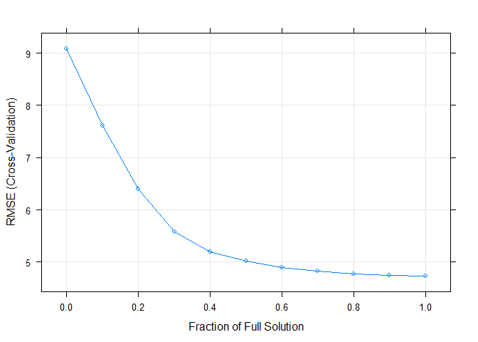
##   0.0       9.075950        NaN  6.651501
##   0.1       7.611127  0.6223092  5.476068
##   0.2       6.399804  0.6449916  4.651807
##   0.3       5.582851  0.6776721  4.047400
##   0.4       5.192926  0.6958606  3.732253
##   0.5       5.022313  0.7111354  3.578952
##   0.6       4.896489  0.7236810  3.482037
##   0.7       4.831206  0.7300803  3.432679
##   0.8       4.776074  0.7358684  3.410385
##   0.9       4.744846  0.7391371  3.408950
##   1.0       4.738682  0.7399459  3.427828
## 
## RMSE was used to select the optimal model using the smallest value.
## The final value used for the model was fraction = 1.

Finally, we can plot the model accross all of the tuning parameters.

plot(model5)