Ridge Regression in R

Intro

Ridge regression is a modified linear regression model called a penalized regression. It adds a penalty to the linear regression model when optimizing to help with multicollinearity issues. In this article, we will learn how to use ridge regression in R.

Data

For this tutorial, we will use the Boston data set which includes housing data with features of the houses and their prices. We would like to predict the medv column or the medium value.

library(MASS)
data(Boston)
str(Boston)

## 'data.frame':    506 obs. of  14 variables:
##  $ crim   : num  0.00632 0.02731 0.02729 0.03237 0.06905 ...
##  $ zn     : num  18 0 0 0 0 0 12.5 12.5 12.5 12.5 ...
##  $ indus  : num  2.31 7.07 7.07 2.18 2.18 2.18 7.87 7.87 7.87 7.87 ...
##  $ chas   : int  0 0 0 0 0 0 0 0 0 0 ...
##  $ nox    : num  0.538 0.469 0.469 0.458 0.458 0.458 0.524 0.524 0.524 0.524 ...
##  $ rm     : num  6.58 6.42 7.18 7 7.15 ...
##  $ age    : num  65.2 78.9 61.1 45.8 54.2 58.7 66.6 96.1 100 85.9 ...
##  $ dis    : num  4.09 4.97 4.97 6.06 6.06 ...
##  $ rad    : int  1 2 2 3 3 3 5 5 5 5 ...
##  $ tax    : num  296 242 242 222 222 222 311 311 311 311 ...
##  $ ptratio: num  15.3 17.8 17.8 18.7 18.7 18.7 15.2 15.2 15.2 15.2 ...
##  $ black  : num  397 397 393 395 397 ...
##  $ lstat  : num  4.98 9.14 4.03 2.94 5.33 ...
##  $ medv   : num  24 21.6 34.7 33.4 36.2 28.7 22.9 27.1 16.5 18.9 ...

Basic Ridge Regression Regression in R

To create a basic ridge regression model in R, we can use the glmnet method from the glmnet package. We set the alpha = 0 to tell glmnet to use ridge.

library(glmnet)

## Warning: package 'glmnet' was built under R version 4.0.5

## Loading required package: Matrix

## Loaded glmnet 4.1-1

predictors = subset(Boston, select = -c(medv))
target = subset(Boston, select = medv)[,1]

model = glmnet(
  x = as.matrix(predictors),
  y = target,
  alpha = 0
)
summary(model)

##           Length Class     Mode   
## a0         100   -none-    numeric
## beta      1300   dgCMatrix S4     
## df         100   -none-    numeric
## dim          2   -none-    numeric
## lambda     100   -none-    numeric
## dev.ratio  100   -none-    numeric
## nulldev      1   -none-    numeric
## npasses      1   -none-    numeric
## jerr         1   -none-    numeric
## offset       1   -none-    logical
## call         4   -none-    call   
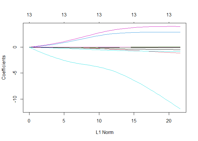
## nobs         1   -none-    numeric

We can plot the model to see how Ridge reduces different ceoffecients on the predictors.

plot(model)

Modeling Ridge Regression in R with Caret

We will now see how to model a ridge regression using the Caret package. We will use this library as it provides us with many features for real life modeling.

To do this, we use the train method. We pass the same parameters as above, but in addition we pass the method = 'ridge' model to tell Caret to use a lasso model.

set.seed(1)

library(caret)

## Loading required package: lattice

## Loading required package: ggplot2

model <- train(
  medv ~ .,
  data = Boston,
  method = 'ridge'
)
model

## Ridge Regression 
## 
## 506 samples
##  13 predictor
## 
## No pre-processing
## Resampling: Bootstrapped (25 reps) 
## Summary of sample sizes: 506, 506, 506, 506, 506, 506, ... 
## Resampling results across tuning parameters:
## 
##   lambda  RMSE      Rsquared   MAE     
##   0e+00   4.914881  0.7152900  3.484317
##   1e-04   4.914758  0.7153023  3.484052
##   1e-01   4.917725  0.7162571  3.412941
## 
## RMSE was used to select the optimal model using the smallest value.
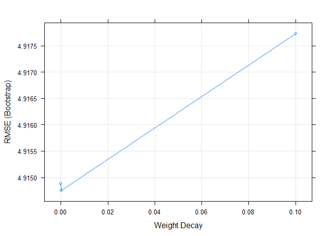
## The final value used for the model was lambda = 1e-04.

Here we can see that caret automatically trained over multiple hyper parameters. We can easily plot those to visualize.

plot(model)

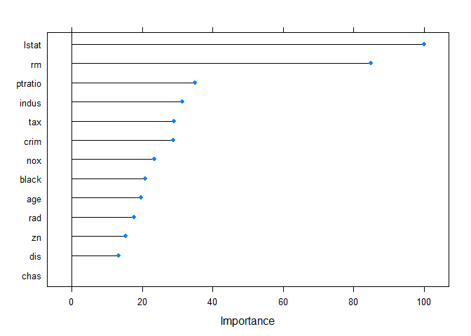
We can also create a variable importance plot to see a ranking of which predictors have more impact.

plot(varImp(model))

Preprocessing with Caret

One feature that we use from Caret is preprocessing. Often in real life data science we want to run some pre processing before modeling. We will center and scale our data by passing the following to the train method: preProcess = c("center", "scale").

set.seed(1)

model2 <- train(
  medv ~ .,
  data = Boston,
  method = 'ridge',
  preProcess = c("center", "scale")
)
model2

## Ridge Regression 
## 
## 506 samples
##  13 predictor
## 
## Pre-processing: centered (13), scaled (13) 
## Resampling: Bootstrapped (25 reps) 
## Summary of sample sizes: 506, 506, 506, 506, 506, 506, ... 
## Resampling results across tuning parameters:
## 
##   lambda  RMSE      Rsquared   MAE     
##   0e+00   4.914881  0.7152900  3.484317
##   1e-04   4.914758  0.7153023  3.484052
##   1e-01   4.917725  0.7162571  3.412941
## 
## RMSE was used to select the optimal model using the smallest value.
## The final value used for the model was lambda = 1e-04.

Splitting the Data Set

Often when we are modeling, we want to split our data into a train and test set. This way, we can check for overfitting. We can use the createDataPartition method to do this. In this example, we use the target medv to split into an 80/20 split, p = .80.

This function will return indexes that contains 80% of the data that we should use for training. We then use the indexes to get our training data from the data set.

set.seed(1)

inTraining <- createDataPartition(Boston$medv, p = .80, list = FALSE)
training <- Boston[inTraining,]
testing  <- Boston[-inTraining,]

We can then fit our model again using only the training data.

set.seed(1)
model3 <- train(
  medv ~ .,
  data = training,
  method = 'ridge',
  preProcess = c("center", "scale")
)
model3

## Ridge Regression 
## 
## 407 samples
##  13 predictor
## 
## Pre-processing: centered (13), scaled (13) 
## Resampling: Bootstrapped (25 reps) 
## Summary of sample sizes: 407, 407, 407, 407, 407, 407, ... 
## Resampling results across tuning parameters:
## 
##   lambda  RMSE      Rsquared   MAE     
##   0e+00   4.895637  0.7167782  3.454826
##   1e-04   4.895610  0.7167819  3.454690
##   1e-01   4.949115  0.7139877  3.440440
## 
## RMSE was used to select the optimal model using the smallest value.
## The final value used for the model was lambda = 1e-04.

Now, we want to check our data on the test set. We can use the subset method to get the features and test target. We then use the predict method passing in our model from above and the test features.

Finally, we calculate the RMSE and r2 to compare to the model above.

test.features = subset(testing, select=-c(medv))
test.target = subset(testing, select=medv)[,1]

predictions = predict(model3, newdata = test.features)

# RMSE
sqrt(mean((test.target - predictions)^2))

## [1] 5.120435

# R2
cor(test.target, predictions) ^ 2

## [1] 0.7126274

Cross Validation

In practice, we don’t normal build our data in on training set. It is common to use a data partitioning strategy like k-fold cross-validation that resamples and splits our data many times. We then train the model on these samples and pick the best model. Caret makes this easy with the trainControl method.

We will use 10-fold cross-validation in this tutorial. To do this we need to pass three parameters method = "cv", number = 10 (for 10-fold). We store this result in a variable.

set.seed(1)
ctrl <- trainControl(
  method = "cv",
  number = 10,
)

Now, we can retrain our model and pass the trainControl response to the trControl parameter. Notice the our call has added trControl = set.seed.

set.seed(1)

model4 <- train(
  medv ~ .,
  data = training,
  method = 'ridge',
  preProcess = c("center", "scale"),
  trControl = ctrl
)
model4

## Ridge Regression 
## 
## 407 samples
##  13 predictor
## 
## Pre-processing: centered (13), scaled (13) 
## Resampling: Cross-Validated (10 fold) 
## Summary of sample sizes: 367, 366, 367, 366, 365, 367, ... 
## Resampling results across tuning parameters:
## 
##   lambda  RMSE      Rsquared   MAE     
##   0e+00   4.738682  0.7399459  3.427828
##   1e-04   4.738608  0.7399540  3.427727
##   1e-01   4.765288  0.7393663  3.414240
## 
## RMSE was used to select the optimal model using the smallest value.
## The final value used for the model was lambda = 1e-04.

This results seemed to have improved our accuracy for our training data. Let’s check this on the test data to see the results.

test.features = subset(testing, select=-c(medv))
test.target = subset(testing, select=medv)[,1]

predictions = predict(model4, newdata = test.features)

# RMSE
sqrt(mean((test.target - predictions)^2))

## [1] 5.120435

# R2
cor(test.target, predictions) ^ 2

## [1] 0.7126274

Tuning Hyper Parameters

To tune a ridge model, we can give the model different values of lambda. Caret will retrain the model using different lambdas and select the best version.

set.seed(1)

tuneGrid <- expand.grid(
  .lambda = seq(0, .1, by = 0.01)
)


model5 <- train(
  medv ~ .,
  data = training,
  method = 'ridge',
  preProcess = c("center", "scale"),
  trControl = ctrl,
  tuneGrid = tuneGrid
)
model5

## Ridge Regression 
## 
## 407 samples
##  13 predictor
## 
## Pre-processing: centered (13), scaled (13) 
## Resampling: Cross-Validated (10 fold) 
## Summary of sample sizes: 367, 366, 367, 366, 365, 367, ... 
## Resampling results across tuning parameters:
## 
##   lambda  RMSE      Rsquared   MAE     
##   0.00    4.738682  0.7399459  3.427828
##   0.01    4.733617  0.7405339  3.419158
##   0.02    4.731912  0.7408108  3.413409
##   0.03    4.732410  0.7408942  3.409016
##   0.04    4.734467  0.7408497  3.405893
##   0.05    4.737699  0.7407168  3.403919
##   0.06    4.741863  0.7405205  3.403654
##   0.07    4.746800  0.7402774  3.405022
##   0.08    4.752398  0.7399990  3.407386
##   0.09    4.758580  0.7396933  3.410556
##   0.10    4.765288  0.7393663  3.414240
## 
## RMSE was used to select the optimal model using the smallest value.
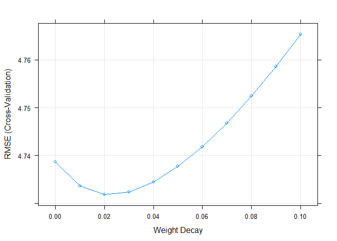
## The final value used for the model was lambda = 0.02.

Finally, we can again plot the model to see how it performs over different tuning parameters.

plot(model5)