
Moving Average in R
07.19.2021
Intro
When working with time series, we often want to view the average over a certain number of days. For example, we can view a 7-day rolling average to give us an idea of change from week to week. In this article, we will learn how to conduct a moving average in R.
Data
Let’s load a data set of monthly milk production. We will load it from the url below. The data consists of monthly intervals and kilograms of milk produced.
df <- read.csv('https://raw.githubusercontent.com/ourcodingclub/CC-time-series/master/monthly_milk.csv')
df$month = as.Date(df$month)
head(df)
## month milk_prod_per_cow_kg
## 1 1962-01-01 265.05
## 2 1962-02-01 252.45
## 3 1962-03-01 288.00
## 4 1962-04-01 295.20
## 5 1962-05-01 327.15
## 6 1962-06-01 313.65Now, we convert our data to a time series object then to an zoo object
to have access to many indexing methods explored below.
library(zoo)##
## Attaching package: 'zoo'
## The following objects are masked from 'package:base':
##
## as.Date, as.Date.numericdf.ts = ts(df[, -1], frequency = 12, start=c(1962, 1, 1))
df.ts = as.zoo(df.ts)
head(df.ts)## Jan 1962 Feb 1962 Mar 1962 Apr 1962 May 1962 Jun 1962
## 265.05 252.45 288.00 295.20 327.15 313.65Conducting a moving average
To conduct a moving average, we can use the rollapply function from
the zoo package. This function takes three variables: the time series,
the number of days to apply, and the function to apply. In the example
below, we run a 2-day mean (or 2 day avg).
library(zoo)
ts.2day.mean = rollapply(df.ts, 2, mean)
head(ts.2day.mean)
## Jan 1962 Feb 1962 Mar 1962 Apr 1962 May 1962 Jun 1962
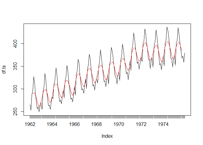
## 258.750 270.225 291.600 311.175 320.400 300.825We can also plot the data over our orignal time series to see how the avg smoothed out the data.
plot(df.ts)
lines(ts.2day.mean, col = 'red')

Let’s do another example with a 7-day avg which is a common task in disease outbreaks and stocks.
ts.7day.mean = rollapply(df.ts, 7, mean)
head(ts.7day.mean)
## Apr 1962 May 1962 Jun 1962 Jul 1962 Aug 1962 Sep 1962
## 289.9286 290.5714 291.0214 286.9714 280.3500 271.0286Again, let’s plot the data.
plot(df.ts)
lines(ts.7day.mean, col = 'red')
Other Rolling Functions
You may have noticed from the above that we can do more than a rolling
average with the rollapply function. We can actually apply any math
function. Let’s run a couple of more examples, sum and median.
ts.7day.median = rollapply(df.ts, 7, median)
head(ts.7day.median)
## Apr 1962 May 1962 Jun 1962 Jul 1962 Aug 1962 Sep 1962
## 288.00 288.00 288.00 288.00 269.55 261.90ts.7day.sum = rollapply(df.ts, 7, sum)
head(ts.7day.sum)## Apr 1962 May 1962 Jun 1962 Jul 1962 Aug 1962 Sep 1962
## 2029.50 2034.00 2037.15 2008.80 1962.45 1897.20