R Random Walk Simuation

Intro

Random walks are one of the fundamental time series models. Despite this simplicity, they are able to model many real world scenarios. In this article, we will learn how to simulate a random walk in R.

What is a Random walk

A random walk is defined that for each observation, we can compute this observation from the last plus some random noise. The equation is as follows:

x_t = x_t − 1 + w_t

The way to read this is, the current value at time t is computed based on the previous value (t - 1) plus some random noise. Where w_t is distributed from normal distribution of mean 0 and 1.

Simulating by Hand

To get a very good understanding, let’s try to simulate this by hand. To start, we need a initial value which we will produce randomly.

Let’s say we ran rnorm(1, mean = 0, sd = 1) and we got the value 1.5. We will use this as our first value, X_1

To get the next value, X_2, we need a W_2 which is the random error for the current step. Again, we can run rnorm(1, mean = 0, sd = 1). Let’s say we get .4. Now, we have the following.

And now we have a small time series [1.5, 1.9]. We can continue this for as long as we want to simulate. Let’s continue that way in code.

Simulating a Random Walk in R

First we will set a seed so that you can reproduce the same results, and we will create a size variable to designate how large of a time series we want to simulate.

set.seed(1)

size <- 200

Next, we will create an empty vector to hold all the data and initialize the first time series entry from a normal distribution.

# Create an empty array to hold our time series
x = numeric(size)

# Create the first value
x[1] <- rnorm(n = 1, mean = 0, sd = 1)

Now, we loop until we have enough variables using the same computation we did above to create a variable at each step.

for (t in 2:size) {
    # Create random noise for this observation
    w.error = rnorm(n = 1, mean = 0, sd = 1)
    
    # Compute the current value based on the previous value and the current noise
    x[t] <- x[t - 1] + w.error
}

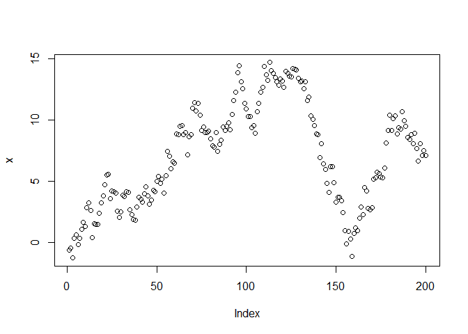
Now, we can plot this data, and we will see a familiar random walk shape.

plot(x)

Simulating with a Library

In practice, we often want simulate a random walk by hand or incrementally in code. Instead, we can use the build in arima.sim function. To do this, we can call the method and pass the model c(0, 1, 0). This stands for 0 AR components, 1 difference component, and 0 MA components.

The details are a bit out of scope for this article, but will be covered in a future post for how to simulate ARIMA models by hand. The only thing to note is that a random walk is 1 difference up from white noise, hence non-stationary.

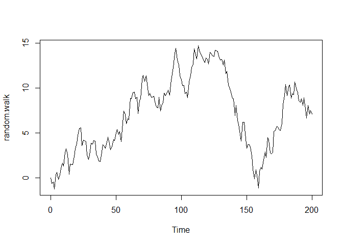
Finally, we pass the number of observations we want to the n parameters

set.seed(1)

random.walk = arima.sim(model = list(order = c(0, 1, 0)), n = 200)

We can end by plotting to see the random walk shape as expected.

plot(random.walk)