
Second Order Exponential Smoothing in R
07.30.2021
Intro
Second Order Exponential Smoothing extends Simple Exponential Smoothing by adding a Trend Smoother. If SES doesn’t work well, we can see if there is a trend and add another component to our model to account for that. In this article, we will learn how to conduct Second Order Exponential Smoothing in R.
Data
Let’s load a data set of monthly milk production. We will load it from the url below. The data consists of monthly intervals and kilograms of milk produced.
df <- read.csv('https://raw.githubusercontent.com/ourcodingclub/CC-time-series/master/monthly_milk.csv')
df$month = as.Date(df$month)
head(df)
## month milk_prod_per_cow_kg
## 1 1962-01-01 265.05
## 2 1962-02-01 252.45
## 3 1962-03-01 288.00
## 4 1962-04-01 295.20
## 5 1962-05-01 327.15
## 6 1962-06-01 313.65Now, we convert our data to a time series object using the R ts
method.
df.ts = ts(df[, -1], frequency = 12, start=c(1962, 1, 1))
head(df.ts)
## [1] 265.05 252.45 288.00 295.20 327.15 313.65Second Order Exponential Smoothing in R"
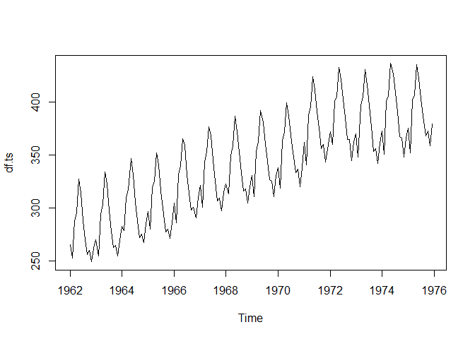
Let’s start by plotting our time series.
plot(df.ts)
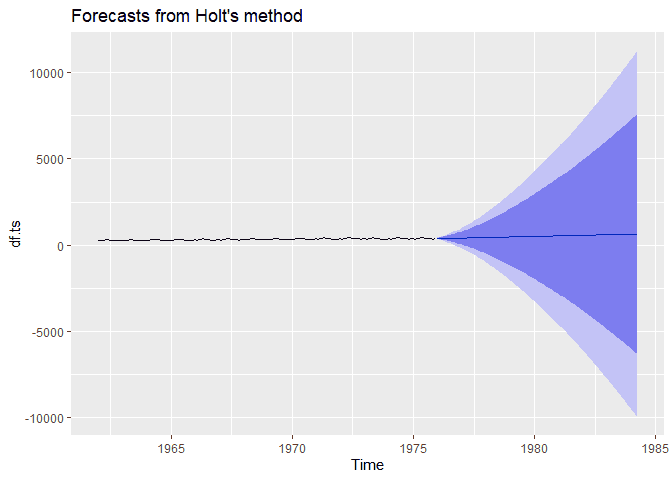
To create a second order exponential smoothing model, we can use the
holt method from the fpp2 package. Here we can pass our time series,
specify a beta value (our trend smoothing parameter), and specify a
horizon h, how many months out (since our data is monthly).
library(fpp2) ## Registered S3 method overwritten by 'quantmod':
## method from
## as.zoo.data.frame zoo
## -- Attaching packages ---------------------------------------------- fpp2 2.4 --
## v ggplot2 3.3.5 v fma 2.4
## v forecast 8.15 v expsmooth 2.3
## ses.ts <- holt(
df.ts,
beta = .4,
h = 100
)
autoplot(ses.ts)
Second Order Exponential Smothing By Hand
Second order exponential smoothing builds on SES by adding a trend component. If you worked through the ses example, you will be able to solve second order with a sligh modificiation.
The equation for SES is the following: Fi + 1 = α**yi + (1 − α)(Fi − Tt − 1)
Where T_t is the trend smothing component defined as follows:
Tt + 1 = β(Ft − Ft − 1) + (1 − β)Tt − 1
Then, we get the predicted value by:
ŷt + 1 = Ft + Tt
Whe initialize the algorithm as follows
To initialize the first trend, we have multiple options. Here are two common ways:
Now, we move to an example. Let’s say we have the following data.
| t | y |
|---|---|
| 1 | 3 |
| 2 | 5 |
| 3 | 9 |
| 4 | 20 |
We can apply our model as follows. We will use an alpha of .4 and beta of .3.
For t = 1.
Now for t = 2.
ŷ2 = F2 + T2 = 4.2 + 1.76 = 5.96
For t = 3
ŷ2 = F2 + T2 = 5.576 + 1.6448 = 7.2208
For t = 4
ŷ2 = F2 + T2 = 7.93248 + 1.858304 = 9.790784 Let’s finish by writing some simple code to replicate this.
y = c(3, 5, 9, 20)

## Start with the first point
forcast = c(y[1])
alpha = .4
beta = .3

# Initialize
F = y[1]
trend = y[2] - y[1]

for (i in 2:length(y)) {
    prev_F = F
    F = alpha * y[i - 1] + (1 - alpha) * (F + trend)
    trend = beta * (F - prev_F) + (1 - beta) * trend
    forcast = append(forcast, F + trend)
}


forcast
## [1] 3.000000 5.960000 7.220800 9.790784