
Second Order Exponential Smoothing in Python
07.29.2021
Intro
Second Order Exponential Smoothing extends Simple Exponential Smoothing by adding a Trend Smoother. If SES doesn't work well, we can see if there is a trend and add another component to our model to account for that. In this article, we will learn how to conduct Second Order Exponential Smoothing in Python.
Data
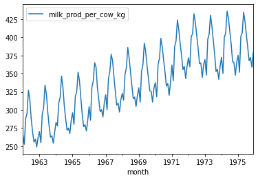
Let's load a data set of monthly milk production. We will load it from the url below. The data consists of monthly intervals and kilograms of milk produced.
import pandas as pd

df = pd.read_csv('https://raw.githubusercontent.com/ourcodingclub/CC-time-series/master/monthly_milk.csv')

df.month = pd.to_datetime(df.month)
df = df.set_index('month')
df.head()| milk_prod_per_cow_kg | |
|---|---|
| month | |
| 1962-01-01 | 265.05 |
| 1962-02-01 | 252.45 |
| 1962-03-01 | 288.00 |
| 1962-04-01 | 295.20 |
| 1962-05-01 | 327.15 |
Simple Exponential Smoothing in Python
Let's start by plotting our time series.
df.plot()<AxesSubplot:xlabel='month'>
To create a simple exponential smoothing model, we can use the Holt from the statsmodels package. We first create an instance of the class with our data, then call the fit method with the value of alpha and beta we want to use. The alpha is the general smoothing level, and the beta is our trend smoothing.
from statsmodels.tsa.api import Holt
import numpy as np

data = df.milk_prod_per_cow_kg

ses = Holt(data)

alpha = 0.4
beta = .3
model = ses.fit(
    smoothing_level = alpha,
    smoothing_trend = beta,
    optimized = False
)
c:\users\krh12\appdata\local\programs\python\python39\lib\site-packages\statsmodels\tsa\base\tsa_model.py:524: ValueWarning: No frequency information was provided, so inferred frequency MS will be used.
warnings.warn('No frequency information was'Now that we have the model, we can forecast using the forcast method. We will predict the next 6 months.
forcast = model.forecast(6)
forcast
c:\users\krh12\appdata\local\programs\python\python39\lib\site-packages\statsmodels\tsa\base\tsa_model.py:132: FutureWarning: The 'freq' argument in Timestamp is deprecated and will be removed in a future version.
date_key = Timestamp(key, freq=base_index.freq)
1976-01-01 363.939243
1976-02-01 358.239791
1976-03-01 352.540340
1976-04-01 346.840888
1976-05-01 341.141436
1976-06-01 335.441985
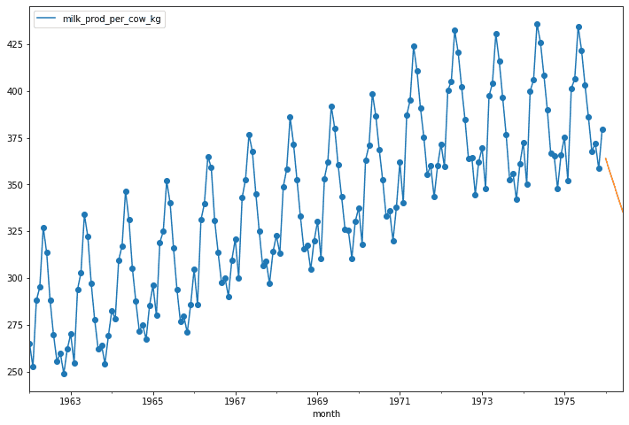
Freq: MS, dtype: float64We can then plot the forcasted with our original data. Unfortunately, the model just predicts three of the same values :P.
ax = data.plot(marker = 'o', figsize = (12,8), legend = True)

forcast.plot(ax = ax)
<AxesSubplot:xlabel='month'>
Second Order Exponential Smothing By Hand
Second order exponential smoothing builds on SES by adding a trend component. If you worked through the ses example, you will be able to solve second order with a sligh modificiation.
The equation for SES is the following:
Where T_t is the trend smothing component defined as follows:
Then, we get the predicted value by:
Whe initialize the algorithm as follows
To initialize the first trend, we have multiple options. Here are two common ways:
Now, we move to an example. Let's say we have the following data.
| t | y |
|---|---|
| 1 | 3 |
| 2 | 5 |
| 3 | 9 |
| 4 | 20 |
We can apply our model as follows. We will use an alpha of .4 and beta of .3.
For t = 1.
Now for t = 2.
For t = 3
For t = 4
Let's finish by writing some simple code to replicate this.
y = [3, 5, 9, 20]

## Start with the first point
forcast = [y[0]]
alpha = .4
beta = .3

# Initialize
F = y[0]
trend = y[1] - y[0]

for i in range(1, len(y)):
    prev_F = F
    F = alpha * y[i - 1] + (1 - alpha) * (F + trend)
    trend = beta * (F - prev_F) + (1 - beta) * trend
    print(F, trend)
    forcast.append(F + trend)

forcast
4.2 1.76
5.5760000000000005 1.6448
7.93248 1.8583039999999997
[3, 5.96, 7.2208000000000006, 9.790784]