SVM Regression in R

Intro

SVM models are a varied model that can work for both regression and classification. They work to find a hyperplance between points and increase the margin. We will leave the math to a different post, but a benifit of this algorithm is it no

Data

For this tutorial, we will use the Boston data set which includes housing data with features of the houses and their prices. We would like to predict the medv column or the medium value.

library(MASS)

data(Boston)

str(Boston)

## 'data.frame':    506 obs. of  14 variables:
##  $ crim   : num  0.00632 0.02731 0.02729 0.03237 0.06905 ...
##  $ zn     : num  18 0 0 0 0 0 12.5 12.5 12.5 12.5 ...
##  $ indus  : num  2.31 7.07 7.07 2.18 2.18 2.18 7.87 7.87 7.87 7.87 ...
##  $ chas   : int  0 0 0 0 0 0 0 0 0 0 ...
##  $ nox    : num  0.538 0.469 0.469 0.458 0.458 0.458 0.524 0.524 0.524 0.524 ...
##  $ rm     : num  6.58 6.42 7.18 7 7.15 ...
##  $ age    : num  65.2 78.9 61.1 45.8 54.2 58.7 66.6 96.1 100 85.9 ...
##  $ dis    : num  4.09 4.97 4.97 6.06 6.06 ...
##  $ rad    : int  1 2 2 3 3 3 5 5 5 5 ...
##  $ tax    : num  296 242 242 222 222 222 311 311 311 311 ...
##  $ ptratio: num  15.3 17.8 17.8 18.7 18.7 18.7 15.2 15.2 15.2 15.2 ...
##  $ black  : num  397 397 393 395 397 ...
##  $ lstat  : num  4.98 9.14 4.03 2.94 5.33 ...
##  $ medv   : num  24 21.6 34.7 33.4 36.2 28.7 22.9 27.1 16.5 18.9 ...

Basic SVM Regression in R

To create a basic svm regression in r, we use the svm method from the e17071 package. We supply two parameters to this method. The first parameter is a formula medv ~ . which means model the medium value parameter by all other parameters. Then, we supply our data set, Boston.

library(e1071)

## Warning: package 'e1071' was built under R version 4.0.5

model = svm(medv ~ ., data = Boston)
print(model)

## 
## Call:
## svm(formula = medv ~ ., data = Boston)
## 
## 
## Parameters:
##    SVM-Type:  eps-regression 
##  SVM-Kernel:  radial 
##        cost:  1 
##       gamma:  0.07692308 
##     epsilon:  0.1 
## 
## 
## Number of Support Vectors:  334

Modeling Linear Regression in R with Caret

We will now see how to model a linear regression using the Caret package. We will use this library as it provides us with many features for real life modeling.

To do this, we use the train method. We pass the same parameters as above, but in addition we pass the method = 'svmRadial' model to tell Caret to use a svm model. Caret also provides us with the fllowing svm options: “svmRadial”, “svmLinear”, or “svmPoly”.

set.seed(1)

library(caret)

## Loading required package: lattice

## Loading required package: ggplot2

library(kernlab)

## 
## Attaching package: 'kernlab'

## The following object is masked from 'package:ggplot2':
## 
##     alpha

model <- train(
  medv ~ .,
  data = Boston,
  method = 'svmRadial'
)
model

## Support Vector Machines with Radial Basis Function Kernel 
## 
## 506 samples
##  13 predictor
## 
## No pre-processing
## Resampling: Bootstrapped (25 reps) 
## Summary of sample sizes: 506, 506, 506, 506, 506, 506, ... 
## Resampling results across tuning parameters:
## 
##   C     RMSE      Rsquared   MAE     
##   0.25  4.698854  0.7612310  2.757942
##   0.50  4.292711  0.7923997  2.554691
##   1.00  3.970728  0.8170827  2.421873
## 
## Tuning parameter 'sigma' was held constant at a value of 0.09566003
## RMSE was used to select the optimal model using the smallest value.
## The final values used for the model were sigma = 0.09566003 and C = 1.

Preprocessing with Caret

One feature that we use from Caret is preprocessing. Often in real life data science we want to run some pre processing before modeling. We will center and scale our data by passing the following to the train method: preProcess = c("center", "scale").

set.seed(1)

model2 <- train(
  medv ~ .,
  data = Boston,
  method = 'svmRadial',
  preProcess = c("center", "scale")
)
model2

## Support Vector Machines with Radial Basis Function Kernel 
## 
## 506 samples
##  13 predictor
## 
## Pre-processing: centered (13), scaled (13) 
## Resampling: Bootstrapped (25 reps) 
## Summary of sample sizes: 506, 506, 506, 506, 506, 506, ... 
## Resampling results across tuning parameters:
## 
##   C     RMSE      Rsquared   MAE     
##   0.25  4.698854  0.7612310  2.757942
##   0.50  4.292711  0.7923997  2.554691
##   1.00  3.970728  0.8170827  2.421873
## 
## Tuning parameter 'sigma' was held constant at a value of 0.09566003
## RMSE was used to select the optimal model using the smallest value.
## The final values used for the model were sigma = 0.09566003 and C = 1.

Splitting the Data Set

Often when we are modeling, we want to split our data into a train and test set. This way, we can check for overfitting. We can use the createDataPartition method to do this. In this example, we use the target medv to split into an 80/20 split, p = .80.

This function will return indexes that contains 80% of the data that we should use for training. We then use the indexes to get our training data from the data set.

set.seed(1)

inTraining <- createDataPartition(Boston$medv, p = .80, list = FALSE)
training <- Boston[inTraining,]
testing  <- Boston[-inTraining,]

set.seed(1)

model3 <- train(
  medv ~ .,
  data = training,
  method = 'svmRadial',
  preProcess = c("center", "scale")
)
model3

## Support Vector Machines with Radial Basis Function Kernel 
## 
## 407 samples
##  13 predictor
## 
## Pre-processing: centered (13), scaled (13) 
## Resampling: Bootstrapped (25 reps) 
## Summary of sample sizes: 407, 407, 407, 407, 407, 407, ... 
## Resampling results across tuning parameters:
## 
##   C     RMSE      Rsquared   MAE     
##   0.25  5.006385  0.7263591  2.959711
##   0.50  4.532278  0.7641084  2.724318
##   1.00  4.183087  0.7908114  2.576319
## 
## Tuning parameter 'sigma' was held constant at a value of 0.1106087
## RMSE was used to select the optimal model using the smallest value.
## The final values used for the model were sigma = 0.1106087 and C = 1.

Now, we want to check our data on the test set. We can use the subset method to get the features and test target. We then use the predict method passing in our model from above and the test features.

Finally, we calculate the RMSE and r2 to compare to the model above.

test.features = subset(testing, select=-c(medv))
test.target = subset(testing, select=medv)[,1]

predictions = predict(model3, newdata = test.features)

# RMSE
sqrt(mean((test.target - predictions)^2))

## [1] 3.825048

# R2
cor(test.target, predictions) ^ 2

## [1] 0.8495157

Cross Validation

In practice, we don’t normal build our data in on training set. It is common to use a data partitioning strategy like k-fold cross-validation that resamples and splits our data many times. We then train the model on these samples and pick the best model. Caret makes this easy with the trainControl method.

We will use 10-fold cross-validation in this tutorial. To do this we need to pass three parameters method = "repeatedcv", number = 10 (for 10-fold). We store this result in a variable.

set.seed(1)
ctrl <- trainControl(
  method = "cv",
  number = 10,
)

Now, we can retrain our model and pass the trainControl response to the trControl parameter. Notice the our call has added trControl = set.seed.

set.seed(1)

model4 <- train(
  medv ~ .,
  data = testing,
  method = 'svmRadial',
  preProcess = c("center", "scale"),
  trCtrl = ctrl
)
model4

## Support Vector Machines with Radial Basis Function Kernel 
## 
## 99 samples
## 13 predictors
## 
## Pre-processing: centered (13), scaled (13) 
## Resampling: Bootstrapped (25 reps) 
## Summary of sample sizes: 99, 99, 99, 99, 99, 99, ... 
## Resampling results across tuning parameters:
## 
##   C     RMSE      Rsquared   MAE     
##   0.25  6.374356  0.5756692  3.771028
##   0.50  5.883662  0.6228022  3.435913
##   1.00  5.455462  0.6646681  3.224363
## 
## Tuning parameter 'sigma' was held constant at a value of 0.08959179
## RMSE was used to select the optimal model using the smallest value.
## The final values used for the model were sigma = 0.08959179 and C = 1.

This results seemed to have improved our accuracy for our training data. Let’s check this on the test data to see the results.

test.features = subset(testing, select=-c(medv))
test.target = subset(testing, select=medv)[,1]

predictions = predict(model4, newdata = test.features)

# RMSE
sqrt(mean((test.target - predictions)^2))

## [1] 3.819472

# R2
cor(test.target, predictions) ^ 2

## [1] 0.8647817

Tuning Hyper Parameters

To tune a svm model, we can give the model different values of C which represents cost and sigma. Caret will retrain the model using different lambdas and select the best version.

set.seed(1)

tuneGrid <- expand.grid(
  C = c(0.25, .5, 1),
  sigma = 0.1
)

model5 <- train(
  medv ~ .,
  data = training,
  method = 'svmRadial',
  preProcess = c("center", "scale"),
  trControl = ctrl,
  tuneGrid = tuneGrid
)
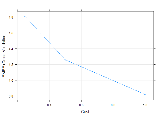
model5

## Support Vector Machines with Radial Basis Function Kernel 
## 
## 407 samples
##  13 predictor
## 
## Pre-processing: centered (13), scaled (13) 
## Resampling: Cross-Validated (10 fold) 
## Summary of sample sizes: 367, 366, 367, 366, 365, 367, ... 
## Resampling results across tuning parameters:
## 
##   C     RMSE      Rsquared   MAE     
##   0.25  4.803438  0.7503886  2.924299
##   0.50  4.258538  0.7930483  2.620436
##   1.00  3.820902  0.8247794  2.409192
## 
## Tuning parameter 'sigma' was held constant at a value of 0.1
## RMSE was used to select the optimal model using the smallest value.
## The final values used for the model were sigma = 0.1 and C = 1.

Finally, we can again plot the model to see how it performs over different tuning parameters.

plot(model5)