
Python Rolling Mean
07.20.2021
Intro
When working with time series, we often want to view the average over a certain number of days. For example, we can view a 7-day rolling average to give us an idea of change from week to week. In this article, we will learn how to conduct a moving average in python.
Data
Let's load a data set of monthly milk production. We will load it from the url below. The data consists of monthly intervals and kilograms of milk produced.
import pandas as pddf = pd.read_csv('https://raw.githubusercontent.com/pandas-dev/pandas/master/doc/data/air_quality_no2_long.csv')df.head()| city | country | date.utc | location | parameter | value | unit | |
|---|---|---|---|---|---|---|---|
| 0 | Paris | FR | 2019-06-21 00:00:00+00:00 | FR04014 | no2 | 20.0 | µg/m³ |
| 1 | Paris | FR | 2019-06-20 23:00:00+00:00 | FR04014 | no2 | 21.8 | µg/m³ |
| 2 | Paris | FR | 2019-06-20 22:00:00+00:00 | FR04014 | no2 | 26.5 | µg/m³ |
| 3 | Paris | FR | 2019-06-20 21:00:00+00:00 | FR04014 | no2 | 24.9 | µg/m³ |
| 4 | Paris | FR | 2019-06-20 20:00:00+00:00 | FR04014 | no2 | 21.4 | µg/m³ |
date_col = 'date.utc'
df = df[[date_col, 'value']]


df[date_col] = pd.to_datetime(df[date_col])
df = df.set_index(date_col)
df = df.sort_index()
C:\Users\krh12\AppData\Local\Temp/ipykernel_13784/1677584757.py:5: SettingWithCopyWarning:
A value is trying to be set on a copy of a slice from a DataFrame.
Try using .loc[row_indexer,col_indexer] = value instead
See the caveats in the documentation: https://pandas.pydata.org/pandas-docs/stable/user_guide/indexing.html#returning-a-view-versus-a-copy
df[date_col] = pd.to_datetime(df[date_col])df.head()| value | |
|---|---|
| date.utc | |
| 2019-05-07 01:00:00+00:00 | 23.0 |
| 2019-05-07 01:00:00+00:00 | 50.5 |
| 2019-05-07 01:00:00+00:00 | 25.0 |
| 2019-05-07 02:00:00+00:00 | 27.7 |
| 2019-05-07 02:00:00+00:00 | 19.0 |
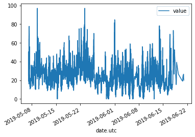
df.plot()<AxesSubplot:xlabel='date.utc'>
Conducting a moving average
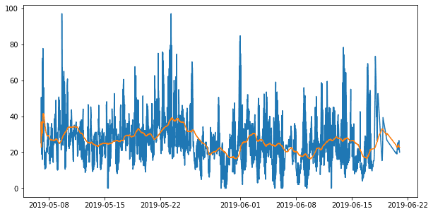
To conduct a moving average, we can use the rolling function from the pandas package that is a method of the DataFrame. This function takes three variables: the time series, the number of days to apply, and the function to apply. In the example below, we run a 2-day mean (or 2 day avg).
twoday_mean = df.rolling('2D').mean()We can also plot the data over our orignal time series to see how the avg smoothed out the data.
import matplotlib.pyplot as plt

fig, ax = plt.subplots(1,1,figsize=(10,5))

ax.plot(df.value)
ax.plot(twoday_mean)

plt.show()
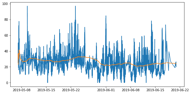
Let's do another example with a 7-day avg which is a common task in disease outbreaks and stocks.
sevenday_mean = df.rolling('7D').mean()
sevenday_mean| value | |
|---|---|
| date.utc | |
| 2019-05-07 01:00:00+00:00 | 23.000000 |
| 2019-05-07 01:00:00+00:00 | 36.750000 |
| 2019-05-07 01:00:00+00:00 | 32.833333 |
| 2019-05-07 02:00:00+00:00 | 31.550000 |
| 2019-05-07 02:00:00+00:00 | 29.040000 |
| ... | ... |
| 2019-06-20 20:00:00+00:00 | 24.443396 |
| 2019-06-20 21:00:00+00:00 | 24.327488 |
| 2019-06-20 22:00:00+00:00 | 24.127143 |
| 2019-06-20 23:00:00+00:00 | 23.900478 |
| 2019-06-21 00:00:00+00:00 | 23.692308 |
2068 rows × 1 columns
import matplotlib.pyplot as plt

fig, ax = plt.subplots(1,1,figsize=(10,5))

ax.plot(df.value)
ax.plot(sevenday_mean)

plt.show()
Other Rolling Functions
You may have noticed from the above that we can do more than a rolling average with the rolling function. We can actually apply any math function. Let's run a couple of more examples, sum and median.
df.rolling('7D').median()| value | |
|---|---|
| date.utc | |
| 2019-05-07 01:00:00+00:00 | 23.00 |
| 2019-05-07 01:00:00+00:00 | 36.75 |
| 2019-05-07 01:00:00+00:00 | 25.00 |
| 2019-05-07 02:00:00+00:00 | 26.35 |
| 2019-05-07 02:00:00+00:00 | 25.00 |
| ... | ... |
| 2019-06-20 20:00:00+00:00 | 18.00 |
| 2019-06-20 21:00:00+00:00 | 18.00 |
| 2019-06-20 22:00:00+00:00 | 18.45 |
| 2019-06-20 23:00:00+00:00 | 18.90 |
| 2019-06-21 00:00:00+00:00 | 18.95 |
2068 rows × 1 columns
df.rolling('7D').sum()| value | |
|---|---|
| date.utc | |
| 2019-05-07 01:00:00+00:00 | 23.0 |
| 2019-05-07 01:00:00+00:00 | 73.5 |
| 2019-05-07 01:00:00+00:00 | 98.5 |
| 2019-05-07 02:00:00+00:00 | 126.2 |
| 2019-05-07 02:00:00+00:00 | 145.2 |
| ... | ... |
| 2019-06-20 20:00:00+00:00 | 5182.0 |
| 2019-06-20 21:00:00+00:00 | 5133.1 |
| 2019-06-20 22:00:00+00:00 | 5066.7 |
| 2019-06-20 23:00:00+00:00 | 4995.2 |
| 2019-06-21 00:00:00+00:00 | 4928.0 |
2068 rows × 1 columns