
Simple Exponential Smoothing in R
07.28.2021
Intro
Simple Exponential Smoothing is a forecasting model that extends the basic moving average by adding weights to previous lags. As the lags grow, the weight, alpha, is decreased which leads to closer lags having more predictive power than farther lags. In this article, we will learn how to create a Simple Exponential Smoothing model in R.
Data
Let’s load a data set of monthly milk production. We will load it from the url below. The data consists of monthly intervals and kilograms of milk produced.
df <- read.csv('https://raw.githubusercontent.com/ourcodingclub/CC-time-series/master/monthly_milk.csv')
df$month = as.Date(df$month)
head(df)
## month milk_prod_per_cow_kg
## 1 1962-01-01 265.05
## 2 1962-02-01 252.45
## 3 1962-03-01 288.00
## 4 1962-04-01 295.20
## 5 1962-05-01 327.15
## 6 1962-06-01 313.65Now, we convert our data to a time series object using the R ts
method.
df.ts = ts(df[, -1], frequency = 12, start=c(1962, 1, 1))
head(df.ts)
## [1] 265.05 252.45 288.00 295.20 327.15 313.65Simple Exponential Smoothing in R
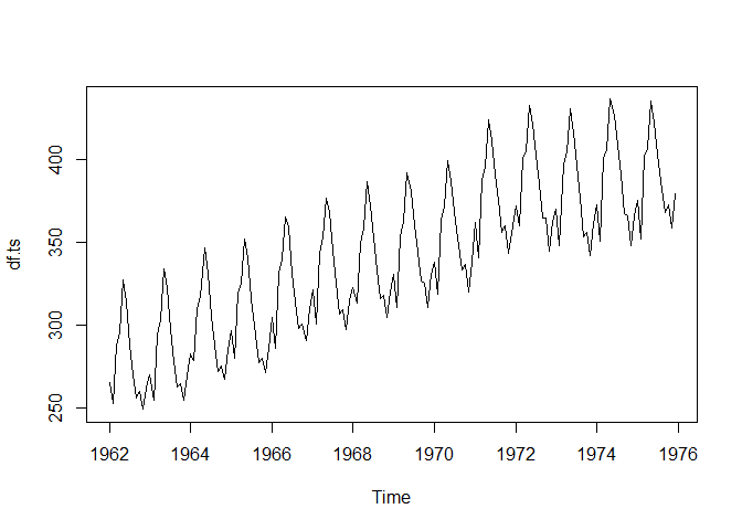
Let’s start by plotting our time series.
plot(df.ts)
To create a simple exponential smoothing model, we can use the
SimpleExpSmoothing from the statsmodels package. We first create an
instance of the class with our data, then call the fit method with the
value of alpha we want to use.
library(fpp2) ## Registered S3 method overwritten by 'quantmod':
## method from
## as.zoo.data.frame zoo
## -- Attaching packages ---------------------------------------------- fpp2 2.4 --
## v ggplot2 3.3.5 v fma 2.4
## v forecast 8.15 v expsmooth 2.3
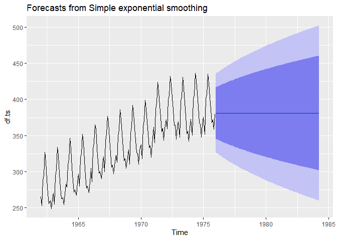
## ses.ts <- ses(df.ts,
alpha = .2,
h = 100)
autoplot(ses.ts)
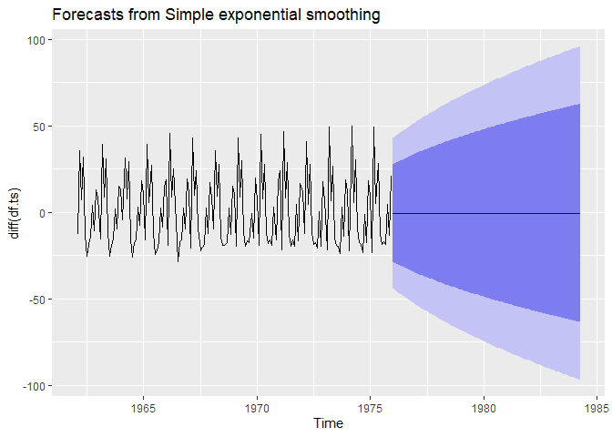
Simple exponential smoothing depends on removing trend and seasonality. We can also use higher order SES methods to remove this. For now, let’s take the first difference and see what happens.
library(fpp2)


ses.ts <- ses(diff(df.ts),
                alpha = .2,
                h = 100)
autoplot(ses.ts)
Simple Exponential Smothing By Hand
SES is a very simple model and helps with understanding future models. With this in mind, I think it is good to try and build these models by hand to help learn the intricate details of models. Learning these simple models will help with the more complex.
The equation for SES is the following:
ŷi + 1 = ŷi + α**ei
You can read this equation by saying, the next value of our time series is the previous value plus alpha (our learning rate) times the error of the previous value.
One this to note is we assume the following:
ŷ1 = y1
That is, the first predicted value is just the first value in our time series.
We can use a bit of algebra to change the equation above to help with iterative calculations. Let’s s.tart with an example of predicting y_3
This gives us a nice form to iterate through an predict data. Let’s see why by doing an example. Let’s say we have the following data.
| t | y |
|---|---|
| 1 | 3 |
| 2 | 5 |
| 3 | 9 |
| 4 | 20 |
We can apply our model as follows. We will use an alpha of .4.
For t = 1.
Now for t = 2.
For t = 3
For t = 4
Let’s finish by writing some simple code to replicate this.
y = c(3, 5, 9, 20)

## Start with the first point
forcast = c(y[1])
alpha = .4


for (i in 2:length(y)) {
  predict = alpha * y[i - 1] + (1 - alpha) * forcast[i - 1]
  forcast = append(forcast, predict)
}


forcast
## [1] 3.00 3.00 3.80 5.88