PCA Regression in R

Intro

PCA or Principal component regression is the process of using PCA to preprocess the data then running a linear regression model. The PCA process will give us new variables or predictors that we can use in modeling. In this article, we will learn how to use pca regression in R.

Data

For this tutorial, we will use the Boston data set which includes housing data with features of the houses and their prices. We would like to predict the medv column or the medium value.

library(MASS)
data(Boston)
str(Boston)

## 'data.frame':    506 obs. of  14 variables:
##  $ crim   : num  0.00632 0.02731 0.02729 0.03237 0.06905 ...
##  $ zn     : num  18 0 0 0 0 0 12.5 12.5 12.5 12.5 ...
##  $ indus  : num  2.31 7.07 7.07 2.18 2.18 2.18 7.87 7.87 7.87 7.87 ...
##  $ chas   : int  0 0 0 0 0 0 0 0 0 0 ...
##  $ nox    : num  0.538 0.469 0.469 0.458 0.458 0.458 0.524 0.524 0.524 0.524 ...
##  $ rm     : num  6.58 6.42 7.18 7 7.15 ...
##  $ age    : num  65.2 78.9 61.1 45.8 54.2 58.7 66.6 96.1 100 85.9 ...
##  $ dis    : num  4.09 4.97 4.97 6.06 6.06 ...
##  $ rad    : int  1 2 2 3 3 3 5 5 5 5 ...
##  $ tax    : num  296 242 242 222 222 222 311 311 311 311 ...
##  $ ptratio: num  15.3 17.8 17.8 18.7 18.7 18.7 15.2 15.2 15.2 15.2 ...
##  $ black  : num  397 397 393 395 397 ...
##  $ lstat  : num  4.98 9.14 4.03 2.94 5.33 ...
##  $ medv   : num  24 21.6 34.7 33.4 36.2 28.7 22.9 27.1 16.5 18.9 ...

Basic PCA Regression in R

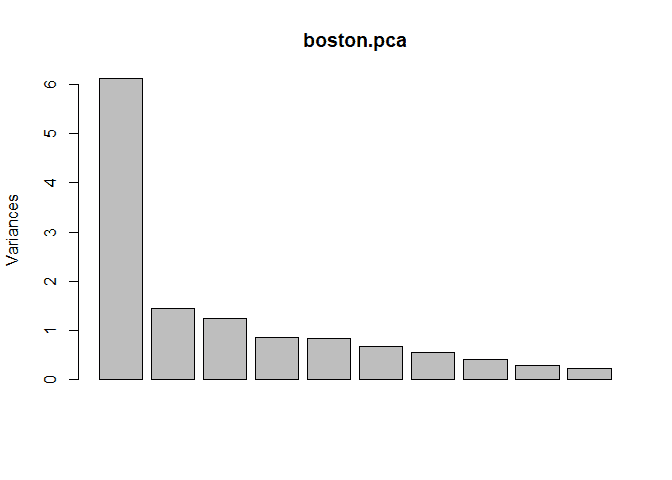
To run pca in R, we can use the built in prcomp function. This will return new variables that are linear combinations of our predictors. We can plot this return to see how much of the variance of our data is examplained by each new predictor.

boston.preds <- subset(Boston, select=-c(medv))
boston.pca <- prcomp(boston.preds, center = TRUE, scale = TRUE)
plot(boston.pca)

To create a pca regression model, we can use the pcr method from the pls package similar to how we run a lm. We pass the model equation, the data set, and we set scale to True so our data will be scaled before building a model.

library(pls)

## Warning: package 'pls' was built under R version 4.0.5

## 
## Attaching package: 'pls'

## The following object is masked from 'package:stats':
## 
##     loadings

model = pcr(medv ~ ., data = Boston, scale = TRUE)
summary(model)

## Data:    X dimension: 506 13 
##  Y dimension: 506 1
## Fit method: svdpc
## Number of components considered: 13
## TRAINING: % variance explained
##       1 comps  2 comps  3 comps  4 comps  5 comps  6 comps  7 comps  8 comps
## X       47.13    58.15    67.71    74.31    80.73    85.79    89.91    92.95
## medv    37.42    45.59    63.59    64.78    69.70    70.05    70.05    70.56
##       9 comps  10 comps  11 comps  12 comps  13 comps
## X       95.08     96.78     98.21     99.51    100.00
## medv    70.57     70.89     71.30     73.21     74.06

Modeling PCA Regression in R with Caret

We will now see how to model a pca regression using the Caret package. We will use this library as it provides us with many features for real life modeling.

To do this, we use the train method. We pass the same parameters as above, but in addition we pass the method = 'lm' model to tell Caret to use a linear model.

As stated before, pca is actually just a processing step. We can pass preProcess = c("pca") to the train method to build a pca model.

library(caret)

## Loading required package: lattice

## Loading required package: ggplot2

## 
## Attaching package: 'caret'

## The following object is masked from 'package:pls':
## 
##     R2

set.seed(1)

model <- train(
  medv ~ .,
  data = Boston,
  method = 'lm',
  preProcess = c("pca")
)
model

## Linear Regression 
## 
## 506 samples
##  13 predictor
## 
## Pre-processing: principal component signal extraction (13), centered
##  (13), scaled (13) 
## Resampling: Bootstrapped (25 reps) 
## Summary of sample sizes: 506, 506, 506, 506, 506, 506, ... 
## Resampling results:
## 
##   RMSE      Rsquared   MAE     
##   5.119009  0.6897642  3.490649
## 
## Tuning parameter 'intercept' was held constant at a value of TRUE

We could use summary again to get extra details. We also see that our RMSE is 5.119009 and our Rsquared is 0.6897642.

Preprocessing with Caret

One feature that we use from Caret is preprocessing. Often in real life data science we want to run some pre processing before modeling. We will center and scale our data by passing the following to the train method: preProcess = c("center", "scale").

set.seed(1)

model2 <- train(
  medv ~ .,
  data = Boston,
  method = 'lm',
  preProcess = c("center", "scale", "pca")
)
model2

## Linear Regression 
## 
## 506 samples
##  13 predictor
## 
## Pre-processing: centered (13), scaled (13), principal component
##  signal extraction (13) 
## Resampling: Bootstrapped (25 reps) 
## Summary of sample sizes: 506, 506, 506, 506, 506, 506, ... 
## Resampling results:
## 
##   RMSE      Rsquared   MAE     
##   5.119009  0.6897642  3.490649
## 
## Tuning parameter 'intercept' was held constant at a value of TRUE

Splitting the Data Set

Often when we are modeling, we want to split our data into a train and test set. This way, we can check for overfitting. We can use the createDataPartition method to do this. In this example, we use the target medv to split into an 80/20 split, p = .80.

This function will return indexes that contains 80% of the data that we should use for training. We then use the indexes to get our training data from the data set.

set.seed(1)

inTraining <- createDataPartition(Boston$medv, p = .80, list = FALSE)
training <- Boston[inTraining,]
testing  <- Boston[-inTraining,]

We can then fit our model again using only the training data.

set.seed(1)
model3 <- train(
  medv ~ .,
  data = training,
  method = 'lm',
  preProcess = c("center", "scale", "pca")
)
model3

## Linear Regression 
## 
## 407 samples
##  13 predictor
## 
## Pre-processing: centered (13), scaled (13), principal component
##  signal extraction (13) 
## Resampling: Bootstrapped (25 reps) 
## Summary of sample sizes: 407, 407, 407, 407, 407, 407, ... 
## Resampling results:
## 
##   RMSE      Rsquared   MAE     
##   5.160234  0.6852131  3.540184
## 
## Tuning parameter 'intercept' was held constant at a value of TRUE

Now, we want to check our data on the test set. We can use the subset method to get the features and test target. We then use the predict method passing in our model from above and the test features.

Finally, we calculate the RMSE and r2 to compare to the model above.

test.features = subset(testing, select=-c(medv))
test.target = subset(testing, select=medv)[,1]

predictions = predict(model3, newdata = test.features)

# RMSE
sqrt(mean((test.target - predictions)^2))

## [1] 5.343331

# R2
cor(test.target, predictions) ^ 2

## [1] 0.6865547

Cross Validation

In practice, we don’t normal build our data in on training set. It is common to use a data partitioning strategy like k-fold cross-validation that resamples and splits our data many times. We then train the model on these samples and pick the best model. Caret makes this easy with the trainControl method.

We will use 10-fold cross-validation in this tutorial. To do this we need to pass three parameters method = "repeatedcv", number = 10 (for 10-fold). We store this result in a variable.

set.seed(1)
ctrl <- trainControl(
  method = "cv",
  number = 10,
)

Now, we can retrain our model and pass the trainControl response to the trControl parameter. Notice the our call has added trControl = set.seed.

set.seed(1)

model4 <- train(
  medv ~ .,
  data = training,
  method = 'lm',
  preProcess = c("center", "scale", "pca"),
  trControl = ctrl
)
model4

## Linear Regression 
## 
## 407 samples
##  13 predictor
## 
## Pre-processing: centered (13), scaled (13), principal component
##  signal extraction (13) 
## Resampling: Cross-Validated (10 fold) 
## Summary of sample sizes: 367, 366, 367, 366, 365, 367, ... 
## Resampling results:
## 
##   RMSE      Rsquared   MAE     
##   4.980723  0.7122785  3.550651
## 
## Tuning parameter 'intercept' was held constant at a value of TRUE

This results seemed to have improved our accuracy for our training data. Let’s check this on the test data to see the results.

test.features = subset(testing, select=-c(medv))
test.target = subset(testing, select=medv)[,1]

predictions = predict(model4, newdata = test.features)

# RMSE
sqrt(mean((test.target - predictions)^2))

## [1] 5.343331

# R2
cor(test.target, predictions) ^ 2

## [1] 0.6865547

Tuning Hyper Parameters

We can also use caret to tune hyper parameters in models. PCA Regression doesn’t have any, so we don’t need to tune the model.